Part 2 · Detection and its evaluation
Day 1 · slides 34–48
Is the detector useful?
Pipeline focus: evaluation.
What you will be able to do
- Calculate precision and daily alert load from detection rate, false-positive rate and base rate.
- Read an ROC curve and justify an operating threshold.
- Check whether analysts can keep up with the queue.
- Treat an explanation as a lead, and combine evidence before acting on an alert.
Follow along
- Slides 34–48 in the browser
- PDF handout (all of Parts 1–3)
On this page: Count the decisions Can analysts keep up? Three alerts, worked through Back to accuracy Self-check Practise Part 2
Count the decisions · slides 35–40
Slide 35 · Misuse or anomaly?

One flow record: workstation ws-114 sends 95 MB/min to 203.0.113.45 at 09:05. Detection objective and training signal are separate axes and do not map one-to-one.
| Misuse detection | Anomaly detection | |
|---|---|---|
| Question | Does it match known malicious behaviour? | Is it unusual for ws-114? |
| Methods | Authored rules or a classifier trained on attack labels | Statistics or a one-class model |
| Here | Known exfiltration signature: none; destination on threat feed: no → no match | z = \frac{95 - 10}{1.225} \approx 69.4 → very unusual |
| Limit | Coverage depends on known evidence. | A backup is also unusual. |
Step by step, as on the slide:
- Misuse detection asks whether the event matches known malicious behaviour. Signatures are one implementation, not the definition. Nothing known matches here.
- Anomaly detection asks whether the event is unusual for ws-114. Its Lab 04 office history has mean \mu = 10 MB/min and \sigma \approx 1.225, so z = (95 - 10)/1.225 \approx 69.4. Anomaly methods need not be unsupervised; one-class training assumes a clean baseline. A scheduled backup is also unusual for an office workstation.
- Neither result proves intent. Check the process, the destination and the job schedule. The objective does not fix the method; the per-entity baselines return on slide 46.
False-alert load and coverage of new attacks depend on features, data, threshold and deployment. Sources: Denning (1987), anomaly model · Kumar & Spafford (1994), misuse model · Sommer & Paxson (2010).
Slides 36–38 · Count decisions → precision → recall and false-positive rate
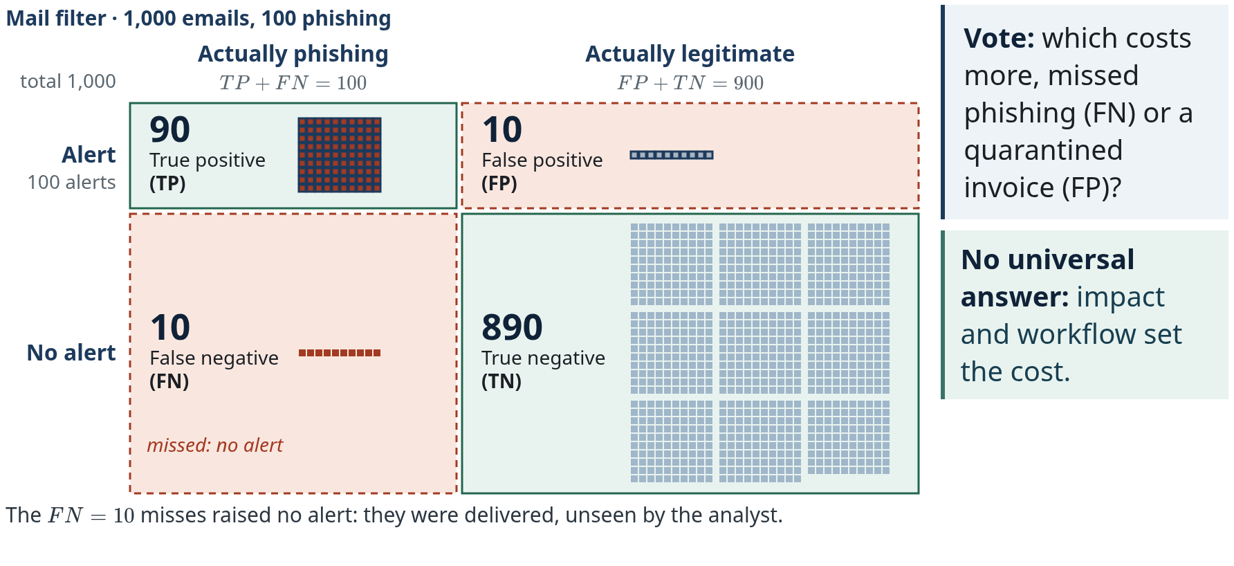
A mail filter at threshold 0.50 over 1,000 emails, 100 of them phishing. Step by step, as on slide 36:
- One square per email: red squares are the 100 phishing emails, grey squares the 900 legitimate ones.
- Every email has two facts: truth and decision. The outlined squares are the filter's 100 alerts: 90 on phishing emails, 10 on legitimate ones.
- Sorted by truth (columns) and decision (rows): TP + FN = 100 phishing emails, FP + TN = 900 legitimate, all = 1{,}000.
- The outlined Alert row is what an analyst sees: TP + FP = 90 + 10 = 100 alerts, and precision divides by it.
- The outline clears and the 10 misses are marked: they were delivered and raised no alert. Later investigation, other controls or audits may still reveal them, and the “actual” labels themselves need evidence.
- Vote: which costs more, missed phishing (FN) or a quarantined invoice (FP)?
- Answer to the vote: no universal answer; impact and workflow set the cost.
| Actually phishing | Actually legitimate | Total | |
|---|---|---|---|
| Alert | TP 90 · true positive | FP 10 · false positive | 100 alerts |
| No alert | FN 10 · false negative | TN 890 · true negative | 900 |
| Total | 100 phishing | 900 legitimate | 1,000 |
Other settings: which error costs more for ransomware on a file server? What about quarantined legal contracts? There is no universal answer: a missed ransomware event (FN) can halt the file server; a false alert that quarantines legal contracts (FP) blocks work. Impact, availability and workflow set the cost.
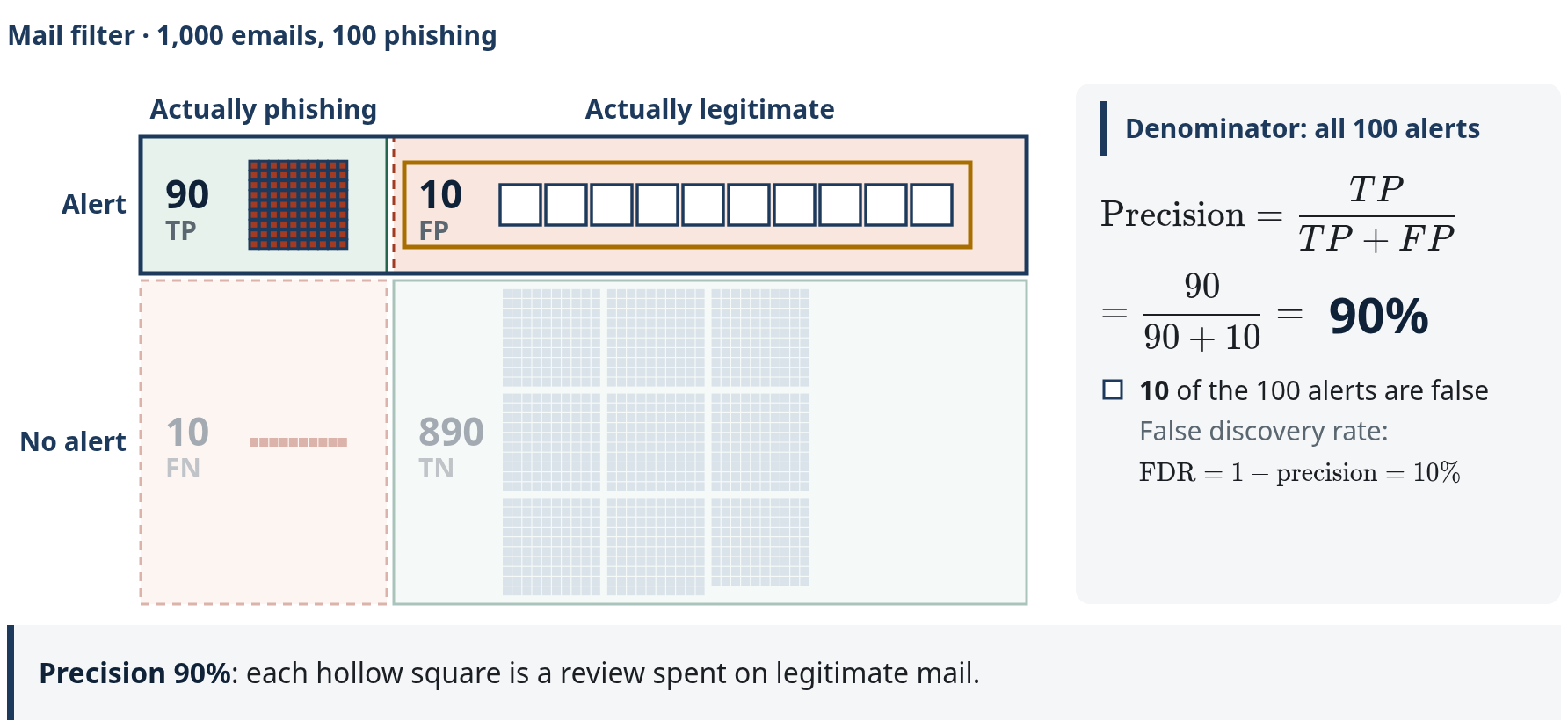
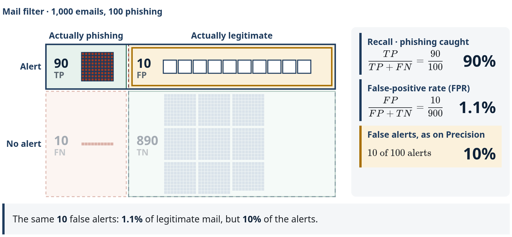
Every metric is a ratio of these cells. Start with the denominator.
Slide 37, step by step:
- The outlined Alert row is the review queue: 90 TP + 10 FP = 100 alerts. Precision divides by these; the 10 FN and 890 TN fade because they never reach review.
- Numerator: TP, the 90 alerts that are real phishing emails. \text{Precision} = \frac{TP}{TP + FP}.
- \frac{90}{90 + 10} = 0.90. The 10 hollow squares are reviews spent on legitimate mail: the false discovery rate, 1 - \text{precision} = 10\%.
Slide 38, step by step:
- Recall: of all the real phishing emails, how many did we catch? Also called detection rate or true-positive rate (TPR); the denominator is the 100 phishing emails. \frac{TP}{TP + FN} = \frac{90}{100} = 90\%; the 10 misses were delivered and raised no alert.
- False-positive rate: the denominator is the 900 legitimate emails. \frac{FP}{FP + TN} = \frac{10}{900} \approx 1.1\%; 890 were delivered. The ROC curve on slide 39 plots one against the other.
- Queue share: the same 10 false alerts are 1.11% of legitimate emails but \frac{FP}{TP + FP} = \frac{10}{100} = 10\% of the alerts: the false discovery rate.
| Measure | Formula | The 1,000 emails | Slide |
|---|---|---|---|
| Precision | \frac{TP}{TP + FP} | \frac{90}{100} = 90\% | 33 |
| Recall / detection rate / TPR | \frac{TP}{TP + FN} | \frac{90}{100} = 90\% | 34 |
| False-positive rate (FPR) | \frac{FP}{FP + TN} | \frac{10}{900} \approx 1.11\% | 34 |
| False discovery rate | \frac{FP}{TP + FP} = 1 - \text{precision} | \frac{10}{100} = 10\% | 33–34 |
| Accuracy | \frac{TP + TN}{\text{all}} | \frac{980}{1{,}000} = 98\% | field guide |
| F_1 | \frac{2\,TP}{2\,TP + FP + FN} | \frac{180}{200} = 90\% | field guide |
Precision and recall both equal 0.90 here because FP and FN happen to be equal; that is not an identity. Accuracy can hide missed rare attacks, and F_1 does not express false-alert workload or the cost of errors. These counts carry a 10% phishing share; the million-event day on slides 39–41 changes the prior, so do not carry 90% precision across. Sources: Fawcett (2006) · Arp et al. (2022), P7.
Slide 39 · What does an ROC curve show?
In plain words: an ROC curve shows every threshold at once. Higher on the curve means more attacks caught; further left means fewer false alerts. The threshold is the score an event needs to raise an alert. A low threshold catches almost everything but floods the queue; a strict one gives about 1,000 false alerts a day, and only about 4 in 100 alerts are real. The AUC (area under the curve) of 0.98 grades the whole curve and hides this.
In detail: a receiver operating characteristic (ROC) curve plots recall against false-positive rate as the threshold t moves. One day has 1,000,000 events and 100 attacks; benign scores follow \mathcal N(0,1) and attack scores \mathcal N(3,1), so
where \Phi is the standard normal distribution function. The slide's x-axis is logarithmic so the low-FPR end, where operations live, is visible.
| Threshold t | FPR | Recall | False alerts/day | Precision |
|---|---|---|---|---|
| 1.0 | 15.87% | 97.7% | \approx 158{,}639 | 0.06% |
| 2.0 | 2.28% | 84.1% | \approx 22{,}748 | 0.37% |
| 3.09 | 0.100% | 46.4% | \approx 1{,}000 | \approx 4.4\% |
Step by step, as on the slide (the interactive version below computes the same points):
- t = 1.0: FPR 15.87%, recall 97.7%. 999{,}900 \cdot 0.1587 \approx 158{,}639 false alerts against about 98 true ones; precision 0.06%.
- t = 3.09, the 99.9th percentile of benign scores (\Phi^{-1}(0.999) = 3.090232): FPR 0.100%, recall 46.4%; about 1,000 false and 46 true alerts, precision 4.4%. \text{AUC} = \Phi(3/\sqrt{2}) \approx 0.983 is one number for the whole curve, the same at every threshold, and it ignores the base rate.
Report recall at a fixed low FPR, or the partial AUC over that range (McClish, 1989), plus precision at the deployment base rate (Davis & Goadrich, 2006). The next slide deliberately uses a different operating point (99% recall, 1% FPR). Sources: Fawcett (2006) · McClish (1989) · Davis & Goadrich (2006).
Slide 40 · Rare attacks, mostly false alerts
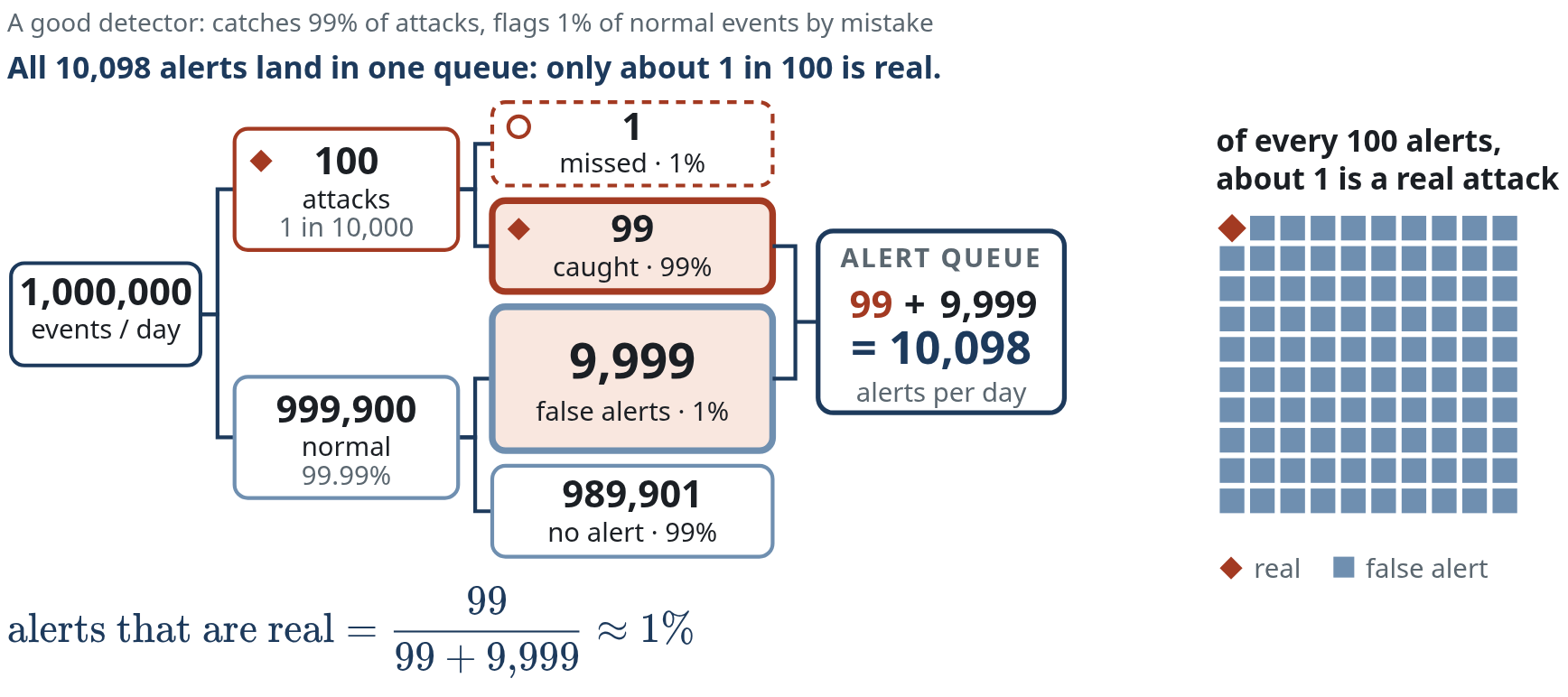
In plain words: a good detector catches 99% of attacks and flags 1% of normal events by mistake. Attacks are rare (1 in 10,000), so the mistakes on the many normal events swamp the few real alerts: only about 1 in 100 alerts is a real attack.
In detail: the base-rate fallacy (Axelsson, 2000); the title states the result. 1,000,000 events/day · 100 attacks. Recall 99% gives 99 true alerts. FPR 1% on 999,900 benign events gives 9,999 false alerts. Precision \approx 1\%: about 99 of every 100 alerts are false. The base rate changes what an alert means. This is a different population from the 1,000 emails: 100 attacks in 1,000,000 events instead of 100 in 1,000, so their 90% precision does not carry over.
Step by step, as on the slide:
- One day: 1,000,000 monitored events, for example sign-ins or process starts, watched by a detector with 99% recall and 1% false-positive rate.
- Split by truth: only 100 of 1,000,000 events are attacks (base rate 0.01%); 999,900 are benign.
- Recall 99% acts on the 100 attacks: 99 alerts, 1 missed.
- FPR 1% acts on 999,900 benign events: 9,999 false alerts; 989,901 benign events raise none. Before the next step: which box makes the title true?
- One queue: 99 + 9{,}999 = 10{,}098 alerts per day, and
the 9,999 false alerts, not the 99 true ones, make the title true. The final caption: all 10,098 alerts land in one queue: only about 1 in 100 is real.
This is Bayes' theorem in counting form, “natural frequencies” (Gigerenzer & Hoffrage, 1995). This day follows Axelsson's argument, not his numbers. His conclusion: the false-positive rate, not the detection rate, is the limiting factor; in his scenario (base rate 2 in 100,000) it must be about 1 in 100,000 for two in three alarms to be real. A score of 0.9 from a model trained on balanced data is not a 90% chance of attack at a 0.01% base rate. Arp et al. (2022) list the base-rate fallacy as pitfall P8. Sources: Axelsson (2000), ACM TISSEC 3(3) · Gigerenzer & Hoffrage (1995) · Arp et al. (2022).
Can analysts keep up? · slides 41–43
Slide 41 · Exercise · how low must the false-positive rate be?
Pairs · 3 minutes. Same day: 1,000,000 events, 100 attacks, recall 99%. Complete the table before opening the answers.
| False-positive rate | False alerts per day | Precision |
|---|---|---|
| 1% | 9,999 | \approx 1\% |
| 0.1% | ? | ? |
| 0.01% | ? | ? |
Answers
FPR 0.1%: 0.001 \cdot 999{,}900 \approx 1{,}000 false alerts against 99 true ones; precision \frac{99}{1{,}099} \approx 9\%. FPR 0.01%: about 100 false alerts against 99 true ones; precision \frac{99}{199} \approx 50\%. Even at one false alarm per 10,000 benign events, about half of all alerts are false. Analyst capacity, not model AUC, sets the usable threshold.
Slide 42 · Live demo · from too many alerts to a workable queue
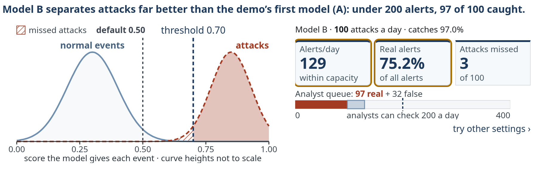
In plain words: on lab data, where 1 in 10 events is an attack, model A looks fine. On real traffic, where 1 in 10,000 is an attack, the same model raises far more alerts than analysts can check. Raising the threshold until analysts can cope means missing 57 of 100 attacks. Only a better model (B) fits within 200 alerts a day and still catches 97 of 100.
In detail: two models score the same events: A (overlapping score distributions) and B (better separated). The SOC can review 200 alerts per day.
| Step | Base rate | Model | Threshold t | Alerts/day | Precision | Missed/day |
|---|---|---|---|---|---|---|
| Start | 10% | A | 0.50 | 139,673 (96,662 true + 43,011 false) | 69.2% | 3,338 |
| 1 | 0.01% | A | 0.50 | 47,883 (97 true + 47,786 false) | 0.2% | 3 |
| 2 | 0.01% | A | 0.74 | 166 (43 true + 123 false) | 26.1% | 57 |
| 3 | 0.01% | B | 0.70 | 129 (97 true + 32 false) | 75.4% | 3 |
Step by step, as on the slide:
- Start, base rate 10%, an enriched lab dataset: model A at 0.50 gives precision about 69%.
- Base rate 0.01%, the day from slide 40: the curves do not move; only the counts behind them change. Precision falls to about 0.2%: roughly 97 true and 48,000 false alerts, 47,883 in total, about 239 times what the SOC can review.
- Raise the threshold to fit capacity: 0.74 is the first value within capacity: 43 + 123 = 166 alerts, precision about 26%, but 57 of 100 attacks per day are missed. At 0.75: 31% and 60 missed. That is the operational price of a low base rate.
- A better-separated model fits capacity and keeps detection: model B at 0.70 detects about 97% of attacks with 97 + 32 = 129 alerts and precision about 75%, 3 missed.
In practice the other levers are analyst capacity and raising the base rate by scoping and correlation. The risk owner, not the vendor default, should decide where the threshold sits. The rate options are assumptions for this demonstration, not universal deployment base rates. Lab 05 lets you repeat this with a concrete queue. Sources: Axelsson (2000) · Alahmadi et al. (2022).
Double events from 1,000 to 2,000 but keep 20 attacks. Why does the queue grow?
There are more benign events to generate false alarms: 99 instead of 49. With 18 true alerts, the queue grows from 67 to 117.
Slide 43 · Analysts cannot review everything
In plain words: 67 alerts arrive in one shift, but there is time to check only 50. If false alerts come first, only 1 of the 18 real attacks gets checked; in random order about 13; if real attacks come first, all 18. The order of the queue decides what gets checked.
- Set thresholds using error costs, review time and capacity: the expected cost of a missed attack, the cost of investigating a false alarm, and alerts per analyst per shift.
- Alert fatigue: SOC practitioners (survey n = 20, interviews n = 21) perceived most alerts as false positives, but most were benign triggers: the rule fired correctly on legitimate activity. Analysts learn to ignore them, may disable noisy rules, and real alerts get buried (Alahmadi et al., 2022). Tuning down a noisy rule is a rational response to low precision, and also how detection coverage erodes.
- Measure the decisions improved, alongside detector performance.
One analyst's shift: 67 alerts against 50 review slots, one analyst's share of the 200 alerts a day on slide 42. Lab 05's rates give the 67: 20 attacks and 980 benign events, recall 90% and FPR 5%, so 0.90 \cdot 20 = 18 true and 0.05 \cdot 980 = 49 false alerts. This is a different population from the 1,000 emails on slide 36. The tiles are grey because the analyst does not yet know which alerts are true. Which 50 get reviewed?
Step by step, as on the slide (the interactive version below draws the same queue):
- Worst order: every false alert first. The 49 false alerts take 49 slots, 17 of the 18 true alerts land outside the slots, and only 1 is reviewed.
- Order unrelated to risk, here the order in which the alerts arrived: 13 true alerts fall inside the slots. The expected value is \mathbb E[\text{true in 50}] = 50 \cdot \frac{18}{67} \approx 13.4.
- Perfect ranking: all 18 true alerts first. This is an upper bound, not a property of this detector. Ranking quality, not only the threshold, decides what capacity buys.
Sources: Alahmadi et al. (2022) · Lab 05.
In the interactive version, Random order draws a different arrival order from each seed: the count inside the 50 slots varies around 13.4.
Three alerts, worked through · slides 44–47
Slide 44 · Alert 1 · a reported email
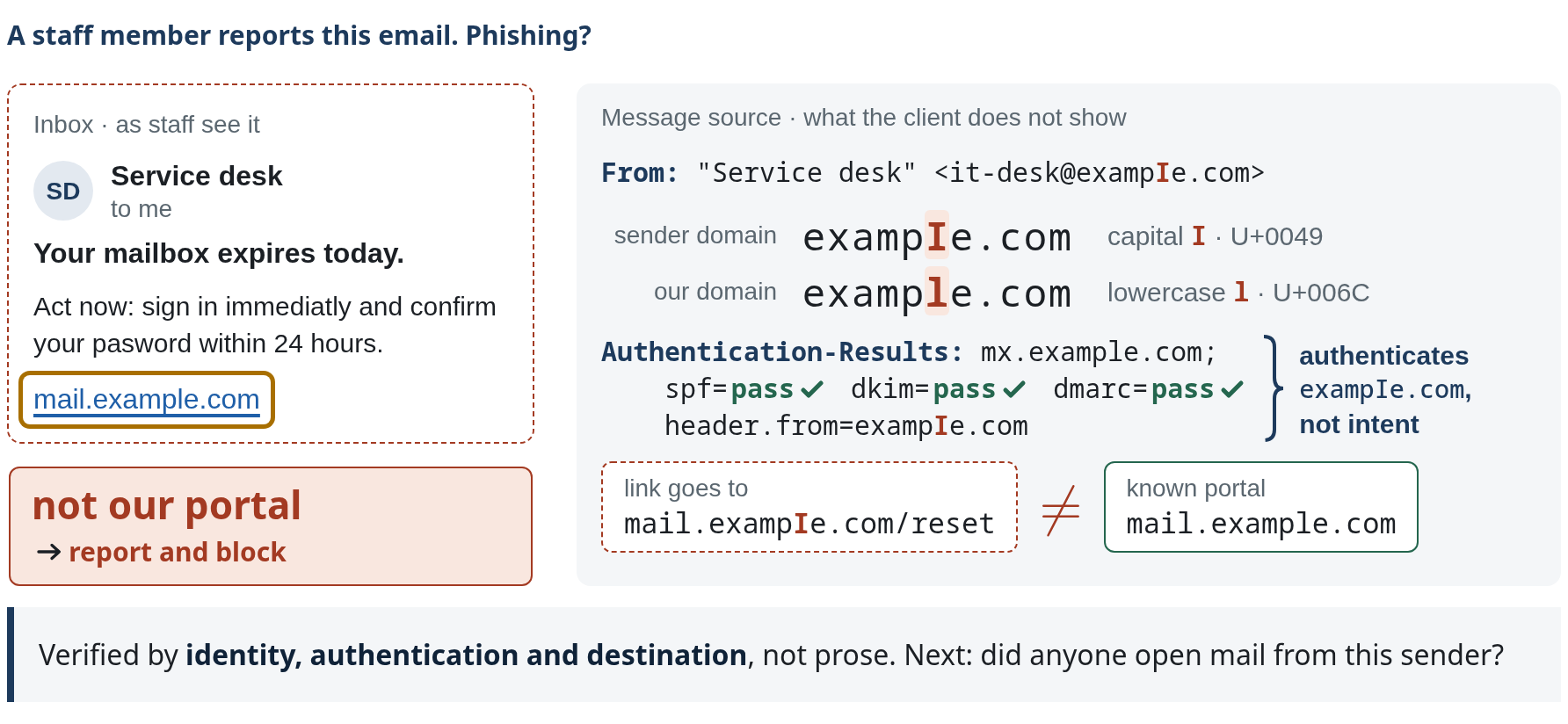
example.com is reserved (RFC 2606); exampIe.com is shown as text only.Slides 44–46 follow one incident through three alerts the analyst checks: an email, an attachment, an upload. A detector is useful only if its alerts can be verified; these slides show what verifying an alert takes. Alert 1 is the phishing email from slide 14, now reported by a staff member. Would you click? An analyst does not judge the prose but opens the message source.
Step by step, as on the slide:
- Identity. “Service desk” is a display name: free text the sender types. The From header carries the address,
it-desk@exampIe.com. - Read the domain letter by letter: “exampIe with a capital I”, U+0049, where
example.comhas a lowercase l, U+006C. In the sans-serif font of a mail client the two are almost identical; in the monospace source they are not. - Authentication. Sender Policy Framework (SPF), DomainKeys Identified Mail (DKIM) and Domain-based Message Authentication, Reporting and Conformance (DMARC) all pass, because the attacker registered
exampIe.comand configured it correctly:Authentication-Results: spf=pass dkim=pass dmarc=pass header.from=exampIe.com. Authentication confirms the message came fromexampIe.com; it says nothing about intent, and a compromised legitimate domain passes as well. - Destination. The link text says
mail.example.com; the target ismail.exampIe.com/reset, which is not the organisation's known portal. Decision: report the message and block the domain. Then: did anyone open mail from this sender? That is alert 2. The final caption: verified by identity, authentication and destination, not prose.
Learned filtering dates back at least to Sahami et al. (1998); for AI-written phishing, rely on the later Heiding study (slide 66), which measures clicks, not compromise (Heiding et al., 2024 [preprint]).
Self-study: train a two-clue phishing classifier and find a mistake its features cannot explain.
After training, why can an approved new portal still raise a false alarm?
Its unfamiliar destination and pressure to sign in resemble the supplied phishing clues. The model does not receive the approval record.
Go deeper with Lab 03 · two fixtures that reverse the pattern
Lab 03 uses the slide-14 representation: link mismatch and credential pressure, with a logistic classifier trained for 500 updates and threshold 0.50.
S1 · trusted site, compromised page. Mismatch 0.05, pressure 0.40. The trained model scores it about 0.061, below 0.50: a miss. A familiar address gives little mismatch even though the page has been compromised.
S3 · approved portal move. Mismatch 0.85, pressure 0.80. The same model flags it: a false alarm on a legitimate migration.
The same feature pattern can correspond to different security outcomes. Training longer cannot make two clues express facts they do not contain. Useful next evidence: who controls the page, site reputation, the organisation's change record and message provenance. Each new feature brings its own collection and reliability questions.
Slide 45 · Alert 2 · the attachment ran
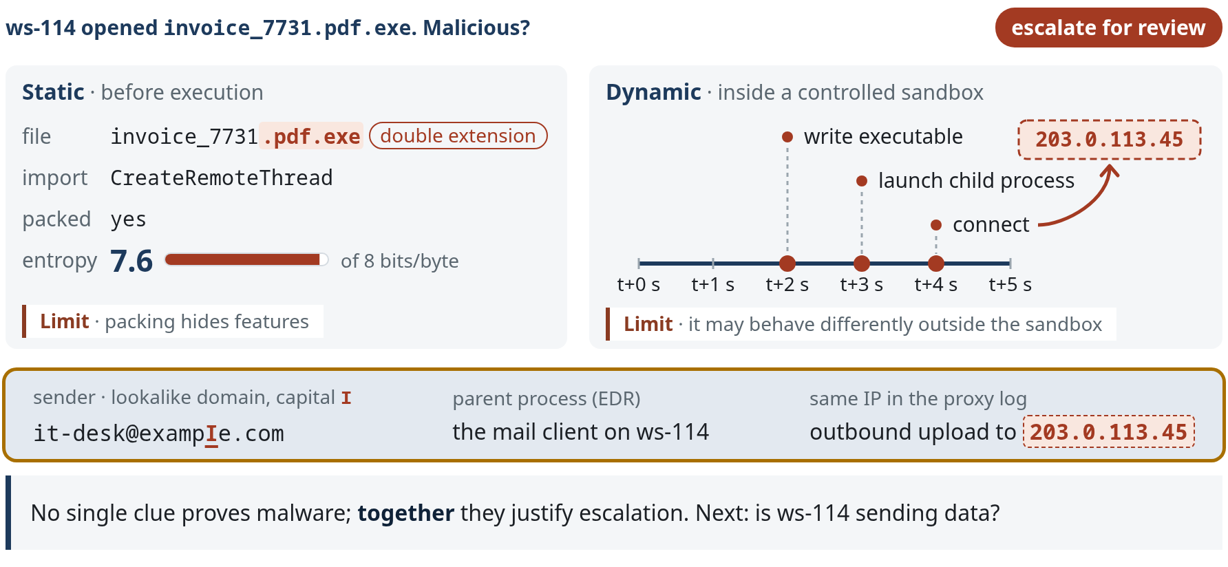
Alert 2: the same sender sent the attachment invoice_7731.pdf.exe, and workstation ws-114 opened it.
Step by step, as on the slide:
- Static inspection reads the file without running it: a double extension, an import of CreateRemoteThread, a packed section with entropy 7.6 of a maximum 8 bits per byte. Importing a thread-creation function is not proof of injection, and benign installers are packed too. Static models can learn the packer as a shortcut instead of the behaviour (Aghakhani et al., 2020). Limit: packing hides features.
- Dynamic inspection runs it in a controlled sandbox: at t+2 s it writes an executable, at t+3 s it launches a child process, at t+4 s it connects to 203.0.113.45, the destination of the ws-114 flow on slide 35. A connection is not proof of command-and-control. Samples can detect the sandbox and delay or alter what they do; Lindorfer et al. (2011) compared behaviour across several analysis sandboxes to find such environment-sensitive samples. Limit: it may behave differently outside the sandbox.
- Three facts from other sources corroborate the clues: the sender is the lookalike domain
it-desk@exampIe.com(capital I); the parent process is the mail client on ws-114, so a user opened the attachment; and the proxy log shows an outbound upload to the same address seen in the sandbox, 203.0.113.45. Together they justify escalating for review; no single clue does.
Labels remain noisy and delayed (Zhu et al., 2020), and new benign software as well as new malware causes drift. Sources: Anderson & Roth (2018) [preprint] · Raff et al. (2018) · Aghakhani et al. (2020) · Lindorfer et al. (2011).
F2 and F4 have the same represented inputs. Can this fixed model give them different scores?
No. Even after adding file-access behaviour, identical represented inputs give the same score. Approval and provenance need other records.
Go deeper with Lab 11 · why entropy alone cannot decide
Byte entropy measures how unpredictable a file's bytes appear; compression and encryption both make it high. File A, a compressed updater, arrives through the managed software channel during an approved maintenance window. File B, a packed executable, arrives as an unsolicited attachment, and an investigation reports access to a customer export and a connection to an unfamiliar destination. Both have high entropy, so entropy alone cannot tell them apart.
Lab 11 trains an entropy-only detector on eight files, then adds a sensitive-behaviour feature and retrains. An approved deployment entry, process/file-access history or destination record would change the judgement; even a signature or an expected filename is not by itself a universal safety verdict. For further study, the Penn State handbook develops malware detection through data and modelling pipelines.
Slide 46 · Alert 3 · the upload from ws-114
- A baseline is specific to a host, user or service.
- Isolation forests separate unusual points: an event that a few random splits isolate from all others is unusual (Liu et al., 2008). Autoencoders learn to compress and rebuild normal traffic and flag traffic they rebuild badly, as in Kitsune (Mirsky et al., 2018).
- The same traffic volume can be unusual for one entity and normal for another.
- Unusual does not establish malicious intent. Dataset artefacts can also inflate evaluations.
Alert 3: ws-114, the workstation that opened the attachment, uploads 95 MB/min to 203.0.113.45, the flow from slide 35. Is that unusual for this host? Each host gets eight observations of outbound traffic from Lab 04, and the score is the distance from that host's own mean in standard deviations (population standard deviation, cutoff 3):
| Host | Observations (MB/min) | \mu | \sigma | z for 95 MB/min |
|---|---|---|---|---|
| ws-114 (office) | 8, 10, 9, 11, 12, 10, 9, 11 | 10 | 1.22 | \frac{85}{1.22} \approx 69.4: unusual |
| Backup server | 80, 92, 100, 108, 95, 105, 90, 110 | 97.5 | 9.54 | \frac{2.5}{9.54} \approx 0.26: normal |
Step by step, as on the slide (the interactive version below builds each baseline one observation per Step):
- Eight observations per host, in MB/min, from Lab 04.
- Each host has its own normal: \mu = 10, \sigma = 1.22 for ws-114; \mu = 97.5, \sigma = 9.54 for the backup server. The band is \mu \pm 3\sigma.
- The same 95 MB/min event lands on both baselines.
- ws-114: z \approx 69.4, unusual. Backup server: z \approx 0.26, ordinary. The anomaly score says “unusual for ws-114”; alone it does not establish intent. With alerts 1 and 2 (the lookalike sender, the attachment opened on ws-114, the same destination) it points to one incident: escalate and request isolation of ws-114 from the authorised approver.
Strengths: no attack labels, and novel behaviour may surface. Weaknesses: benign change is constant, per-entity baselines are noisy, and results are hard to explain. Many published intrusion-detection results were later shown to exploit artefacts of how public datasets were generated (McHugh, 2000; Engelen et al., 2021). Arp et al. (2022) re-evaluated Kitsune on its own Mirai data: a one-feature boxplot of packet rate reached 0.996 detection at 0.1% FPR against Kitsune's 0.882, because the attack was overly conspicuous (pitfalls P6 and P9). Sources: Liu et al. (2008) · Mirsky et al. (2018) · McHugh (2000) · Engelen et al. (2021).
In the interactive version, Host switches between ws-114 and the backup server.
Why does the slow unauthorised transfer escape the office volume check?
Its 12 MB/min rate is near the office reference. A volume-only detector does not receive the accessed files, destination or permission records.
Go deeper with Lab 04 · distance from a baseline
Lab 04 fits a mean and spread (standard deviation) to eight historical measurements per machine and flags an event when its absolute distance |z| = |x - \mu| \div \sigma exceeds a cutoff of 3, a teaching choice.
Office workstation: mean 10 MB/min, spread about 1.225. A 12 MB/min event: (12 - 10) \div 1.225 \approx 1.6 \lt 3, not flagged. Not anomalous does not mean authorised.
Backup server: mean 97.5 MB/min, spread about 9.54. The same 95 MB/min event that is far from the office baseline looks ordinary here: only the reference has changed.
Historical data may be contaminated or no longer representative, and TCP/443 with a high volume does not establish authorisation. Process identity, accessed data, destination and approval records distinguish an approved backup from an unapproved export.
Slide 47 · Explanations are leads, not proof
- Interpretability can be built into rules, small trees and linear models.
- Post-hoc methods assign each feature a share of the difference between this score and a baseline score; the assignment depends on the method's assumptions and is not causal proof.
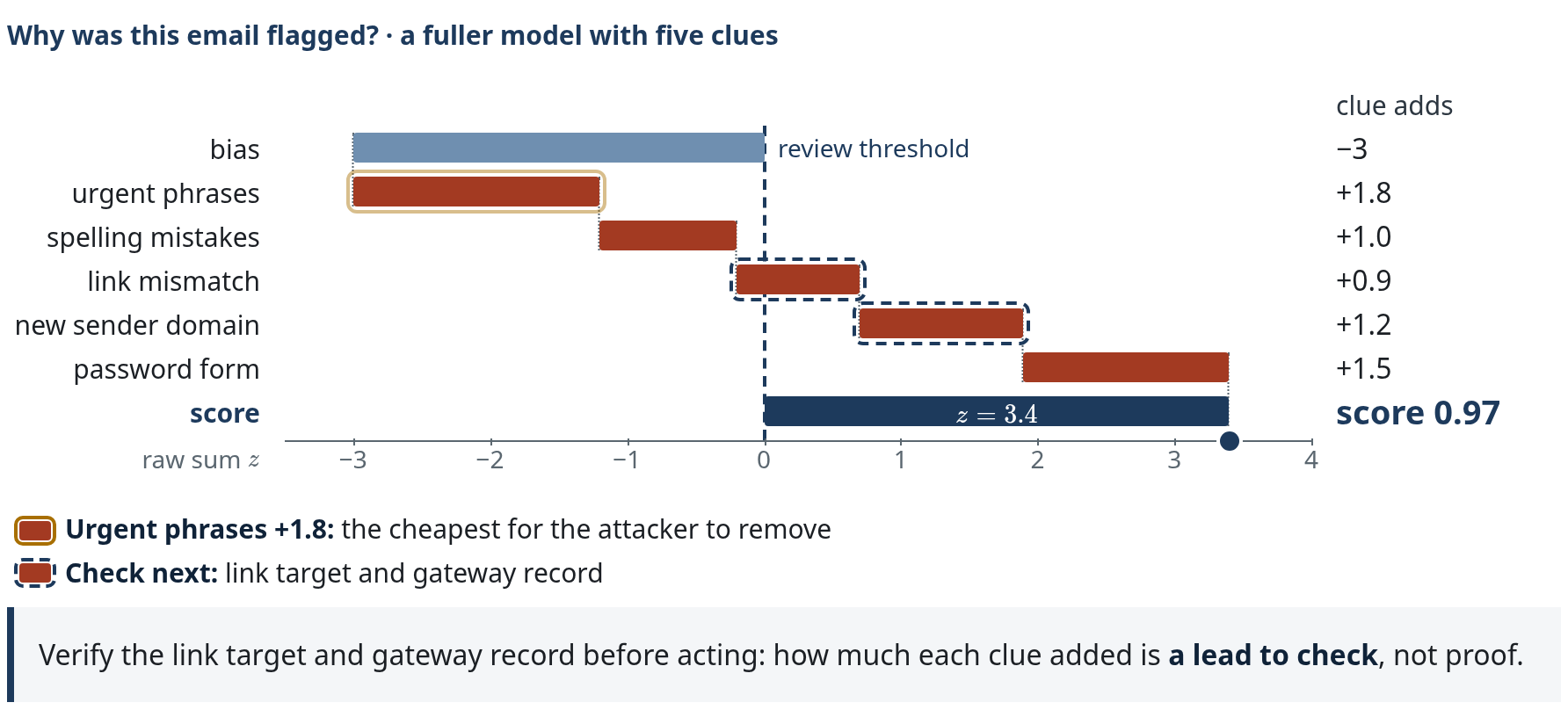
Why did the gateway flag the “Your mailbox expires today.” email? This is gateway v2, the five-feature production model announced on slide 27. The axis is log-odds z; the score is \sigma(z). The review threshold is z = 0, \sigma(0) = 0.50. For a logistic model the additive decomposition lives in log-odds, not in the 0 to 1 score.
Step by step, as on the slide:
- Start from the bias b = -3, the log-odds of an email with none of the features, f(\mathbf 0); score 0.05.
- Each contribution is \phi_j = w_j x_j. Three urgent phrases at weight 0.6 give +1.8; two spelling mistakes at 0.5 give +1.0. The running total is -0.2, still below the threshold.
- Link mismatch +0.9 and new sender domain +1.2: the running total passes the threshold. The order is for display; a running total is not the verdict of any single feature.
- Password form +1.5 completes it: z = -3 + 1.8 + 1.0 + 0.9 + 1.2 + 1.5 = 3.4 and \sigma(3.4) = 0.97, review. The decomposition is exact, \sum_j \phi_j = f(\mathbf x) - f(\mathbf 0), which is SHAP's local accuracy with the all-zero email as the reference (Lundberg & Lee, 2017). A different reference gives different contributions; for nonlinear models SHAP and LIME only estimate them.
- First reading: the largest feature contribution, urgent phrases (+1.8), is the cheapest for the attacker to remove. An evasion attack rephrases exactly these.
- Second reading: the bars to verify are the link mismatch and the new domain. Check the link target and the gateway record from slide 44. Explanations are leads, not proof.
Explanations approximate the model; they can be unfaithful, unstable and even deliberately manipulated (Slack et al., 2020). In a security comparison, gradient-based methods were more accurate and stable (Warnecke et al., 2020). A good explanation tells the analyst which evidence to check next. Sources: Lundberg & Lee (2017) · Lundberg et al. (2020) · Ribeiro et al. (2016) · Guo et al. (2018) · Warnecke et al. (2020) · Slack et al. (2020).
Back to accuracy · slide 48
Slide 48 · Is 99.9% accuracy good?
Question. A vendor tells you its new network detector is “99.9% accurate”. Would you buy it? Which three questions would you ask first, before believing the claim is relevant to your organisation? The slide's answer chips: alert load at our base rate? Whose data, when? Drift and adaptive attackers?
Counter-example and expected questions
On the million-event day of slide 40, a detector that never alerts is \frac{999{,}900}{1{,}000{,}000} = 99.99\% accurate, so accuracy alone answers none of the questions. Ask instead: (1) operating point and alert load: detection rate and false-positive rate at the chosen threshold, and alerts per day for an environment of your size; (2) evaluation data and time split: whose network, which period, temporally separated from training, realistic attack proportion; (3) drift and an adaptive attacker: how performance changes over time, how retraining is handled, and how it behaves against an attacker who knows it is there.
Part 2 answer · Is the detector useful? For analyst triage: only if precision at our base rate fits capacity.
The scope matters: correlated low-precision clues (slide 45) and inline blocking are judged on other terms, such as the cost of a wrong block. Accuracy, AUC and a vendor's headline number do not answer the question.
Self-check · Part 2
A mail filter produces TP 90 and FP 10. What is its precision?
\frac{90}{90 + 10} = 90\%. The denominator is the alerts in the queue.
Why is the false-positive rate multiplied by the number of benign events, not by all events?
FPR is the fraction of benign events that are flagged: \frac{FP}{FP + TN}. On slide 40, 1% of 999,900 benign events gives 9,999 false alerts.
At 1,000,000 events/day with 100 attacks, how many false alerts does an FPR of 0.1% produce?
About 0.001 \cdot 999{,}900 \approx 1{,}000 per day. Precision then depends on recall: about 9% at 99% recall (slide 41), about 4.4% at 46.4% recall (slide 39).
Why can \mathrm{AUC} \approx 0.98 coexist with precision below 5%?
AUC summarises the whole ROC curve and ignores both the base rate and the chosen operating point. At the 0.01% base rate on slide 39, the marked threshold (t = 3.09) gives precision of only about 4.4%, although \mathrm{AUC} \approx 0.98. Raising the threshold improves precision but recall collapses (t = 4: precision \approx 33\%, recall \approx 16\%).
ws-114 sends 95 MB/min. Why is that unusual for ws-114 but not for the backup server?
Each baseline belongs to its entity: z \approx 69.4 against ws-114's mean of 10 MB/min, z \approx 0.26 against the backup server's mean of 97.5 MB/min (slide 46). Neither score establishes intent; the process and destination do.
Practise Part 2
Notebook: Lesson 3 · Investigate behaviour and workload. Worked examples: Lesson 3.