Part 1 · Machine-learning foundations
Day 1 · slides 12–33
How does a model learn from data?
Pipeline focus: data collection · labelling · representation · training.
What you will be able to do
- Explain how supervised and unsupervised learning turn security data into a detector, and what the choice of representation implies.
- Tell the four sources of training signal apart: labels, structure, hidden fields and rewards.
- Say what training changes and what moving a threshold changes.
- Use validation data to catch overfitting.
Follow along
- Slides 12–33 in the browser
- PDF handout (all of Parts 1–3)
On this page: Why this matters What machine learning is Four sources of training signal From data to a detector How a model learns Self-check Practise Part 1
Why this matters · slides 10–11
Slide 10 · Three ways AI meets security
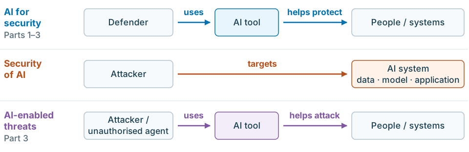
Read the three lanes left to right. In the first and third lanes the AI tool sits in the same position; only the user and the purpose change. In the middle lane the AI system itself is the target. These are actor–action relationships, not a data-flow architecture.
Step by step, as on the slide:
- AI for security. A defender uses an AI tool to help protect people and systems: Parts 1–3.
- Security of AI. The AI system itself is the target: its data, model or application. A defensive detector is itself an AI system that can be attacked.
- AI-enabled threats. The AI tool sits in the same position as in the first lane; only the user and the purpose change.
- Real case · Hugging Face, July 2026. Evaluation agents carried out an unauthorised intrusion into an AI platform; Hugging Face reports using AI to detect and analyse it. One incident touches all three relationships. The actors came from internal evaluations, not an attributed criminal campaign; the defensive-use account is the victim's own, with no independent performance comparison. Slide 68 gives the technical detail.
| AI for security | Security of AI | AI-enabled threats | |
|---|---|---|---|
| Role of AI | Defensive tool | Target / asset | Offensive tool |
| Examples | Malware and phishing detection, anomaly detection, alert triage, threat-intelligence extraction | Evasion, data poisoning, model extraction, prompt injection | Phishing at scale, deepfake fraud, automated reconnaissance and exploitation |
| Covered | Parts 1–3 | not today | Part 3 |
AI is dual-use: the same capability, such as code analysis, serves defender and attacker. Case sources: Hugging Face (16 July 2026) · METR / Redwood (26 August 2026).
Which of the three relationships do you meet most in your own work?
A reflection question with no single answer. Many practitioners meet AI for security through vendor products, and increasingly meet security of AI as organisations deploy LLM assistants.
Slide 11 · Why machine learning in security?
- Scale and variation: large volumes of changing malware, messages and events. AV-TEST registers over 450,000 new malware samples and potentially unwanted applications per day (AV-TEST statistics, accessed October 2026). For vulnerabilities exploited in 2023, Mandiant reports an average time-to-exploit of 5 days, excluding 15 outliers (47 days with them) (Mandiant, 2024).
- Models can generalise and prioritise attention; the threshold on the model's scores, with event volume and base rate, sets the alert load.
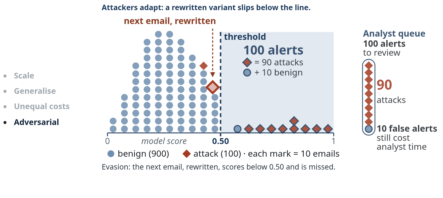
- Adversarial: attackers adapt to the detector.
- Errors have unequal costs: a missed intrusion \neq a false alert.
Step by step, as on the slide:
- 1,000 emails arrive, 100 of them phishing, one dot per 10 emails. Nothing yet separates them. Which deserve an analyst's attention?
- The model scores every email; most phishing emails score high, most benign emails low, with some overlap. A deployed detector sees only the score, not the colours.
- A threshold at 0.50, the same threshold as the email example in Part 1, turns scores into alerts: 100 alerts = 90 attacks + 10 benign emails. Ten phishing emails score below the line and are missed.
- Every alert joins the analyst queue, the 10 false ones too. Event volume, base rate, the model's score distributions and the threshold together set the queue length (Axelsson, 2000).
- Attackers adapt: a rewritten variant slips below the threshold and becomes another miss; the queue fades so the rewritten email stands alone. This is evasion (Biggio & Roli, 2018).
Part 2 returns to exactly these counts and asks whether \text{precision} = \frac{90}{90+10} would still hold on a day of 1,000,000 events with 100 attacks. Sommer and Paxson's argument also returns there: machine learning is good at finding things similar to what it has seen, while intrusion detection often needs the opposite (Sommer & Paxson, 2010).
What machine learning is · slides 13–16
Slide 13 · What is machine learning?
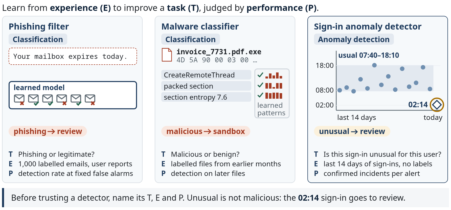
A program learns from experience (E) with respect to a task (T) if its performance (P) at that task improves with experience (Mitchell, 1997). Making T, E and P explicit is the quickest way to make a vendor claim concrete: ask what the task is, what the system learned from, and how it is judged. P must be chosen with the operation in mind: accuracy is almost never the right P in security (Part 2).
| Phishing filter | Malware classifier | Sign-in anomaly detector | |
|---|---|---|---|
| T · task | Phishing or legitimate? | Malicious or benign? | Is this sign-in unusual for this user? |
| E · learn from | 1,000 labelled emails, user reports | Labelled files from earlier months | The user's last 14 days of sign-ins |
| P · check | Detection rate at fixed false alarms | Detection on later files | Confirmed incidents per alert |
Step by step, as on the slide:
- Phishing filter (classification). A new email says “Your mailbox expires today.” A model learned from labelled emails and user reports sends it to review. Slide 14 shows what the model sees in this email and how it scores it.
- Malware classifier (also classification): it labels a file from learned patterns in its features. The attachment
invoice_7731.pdf.exeimports CreateRemoteThread, has a packed section and a section entropy of 7.6. Each feature matches a pattern learned from labelled malware, so the file goes to the sandbox. P uses later files, never the months it learned from. - Sign-in anomaly detector (anomaly detection). There are no attack labels. It learns the user's usual sign-in hours over 14 days, 07:40 to 18:10. Today's sign-in at 02:14 lands outside that band, so it is unusual and goes to review. Unusual is not malicious.
The final caption: before trusting a detector, name its T, E and P.
Slide 14 · One email, a rule and a model
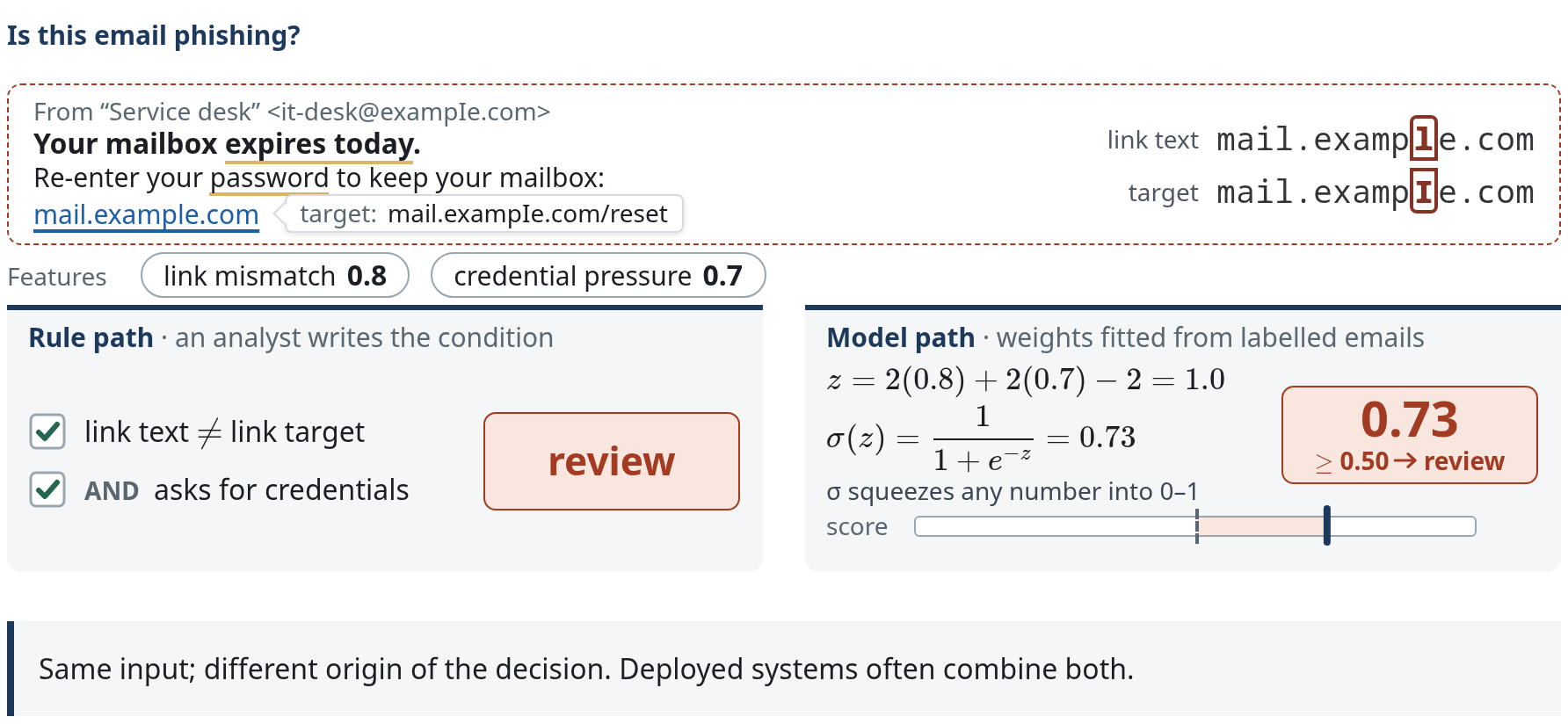
One phishing email, traced through a hand-written rule and through a learned model.
Step by step, as on the slide:
- The email as the user sees it: a familiar sender, an urgent request, a familiar link. Would you click?
- Hovering shows the link target. In monospace the capital I stands apart from the lowercase l: U+0049 against U+006C. Text
mail.example.comand targetmail.exampIe.comdiffer, so link mismatch is 0.8. - Urgency (“expires today”) and a password request give credential pressure 0.7. Checking for a credential request may need the landing page, not only the URL.
- Rule path. An analyst wrote: link text differs from link target AND asks for credentials. Both conditions hold, so review: a yes/no decision with no score.
- Model path. The model weighs the same two features with weights fitted from labelled emails: z = 2(0.8) + 2(0.7) - 2 = 1.0 and \sigma(1.0) = 0.73, above the 0.50 threshold, so review. The sigmoid \sigma(z) = \frac{1}{1 + e^{-z}} squeezes any total into the range 0 to 1.
- Three levers: edit the rule gives a new rule; retraining on new labels gives a new model; moving the threshold changes only the action, never the score.
The input is the same; only the origin of the decision function differs. Deployed systems often combine both (Google, Rules of ML #3, prefer ML to a complex heuristic, and #7, turn heuristics into features). Learning does not mean better: both paths need evaluation. A score of 0.73 is a ranking value; calling it a 73% attack probability would need calibration evidence. How the weights are fitted follows on slides 29–30.
Slide 15 · A model is a learned rule
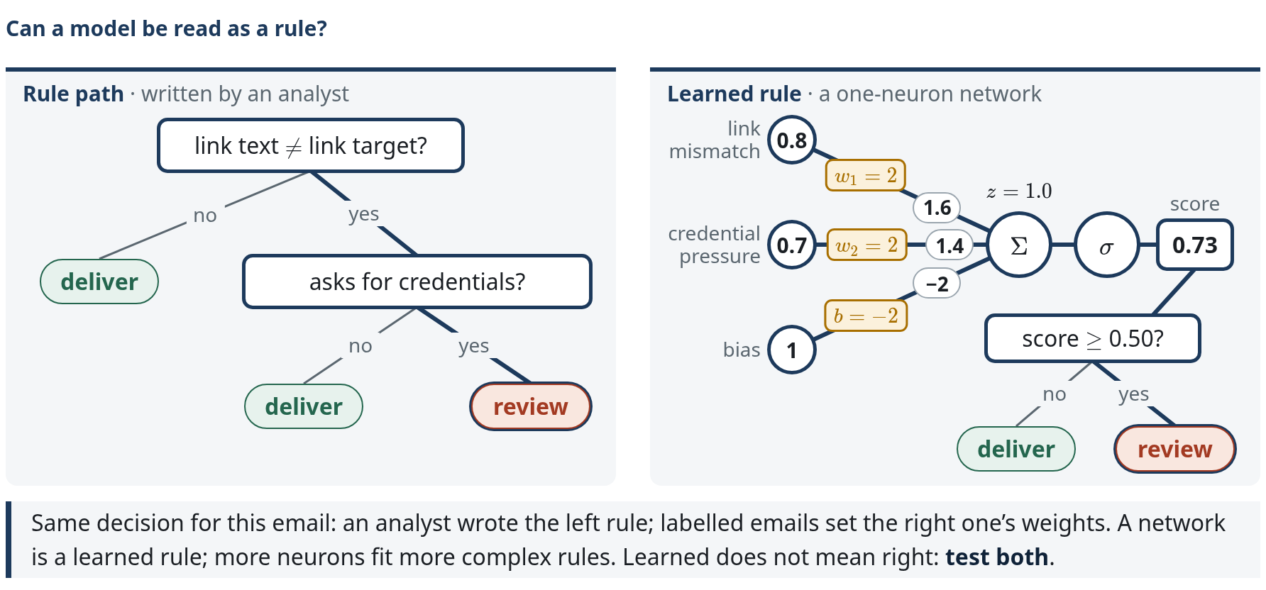
The analyst's rule from slide 14, drawn as a decision tree, beside the fitted model drawn as the smallest neural network: one neuron.
Step by step, as on the slide:
- An analyst's rule and a fitted model both said review. Can the model be drawn like the rule?
- The rule as a tree: two yes/no questions, both chosen by an analyst. Does the link text differ from the link target? No: deliver. Yes: does it ask for credentials? Yes: review; no: deliver.
- Our email: the text says
mail.example.com, the target ismail.exampIe.com, so yes; it asks for a password, so yes: review. - The fitted model as a network: each feature arrives on an edge with a weight, w_1 = 2 and w_2 = 2, and a constant input 1 carries the bias b = -2. No person chose these numbers; they were learned from labelled emails.
- Same email: z = 2(0.8) + 2(0.7) - 2 = 1.0, \sigma(z) = 0.73 \geq 0.50, so review.
- Same decision: an analyst wrote the left rule; labelled emails set the right one's weights. A network is a learned rule; more neurons fit more complex rules. Learned does not mean right: test both, which slide 16 takes up.
The network is exactly the logistic model of slide 14, not an approximation: one sigmoid neuron is logistic regression. Its boundary x_1 + x_2 \geq 1 is a diagonal line, which a tree of yes/no questions on single features can only approximate. Networks with more neurons and layers can fit far more complex boundaries.
Takeaway: a rule and a model make the same kind of decision; what differs is who chose the questions and the numbers. Both still need testing on the same future data.
Sources: Goodfellow et al. (2016) §6.4.1, universal approximation.
Slide 16 · Rules or models? Test both
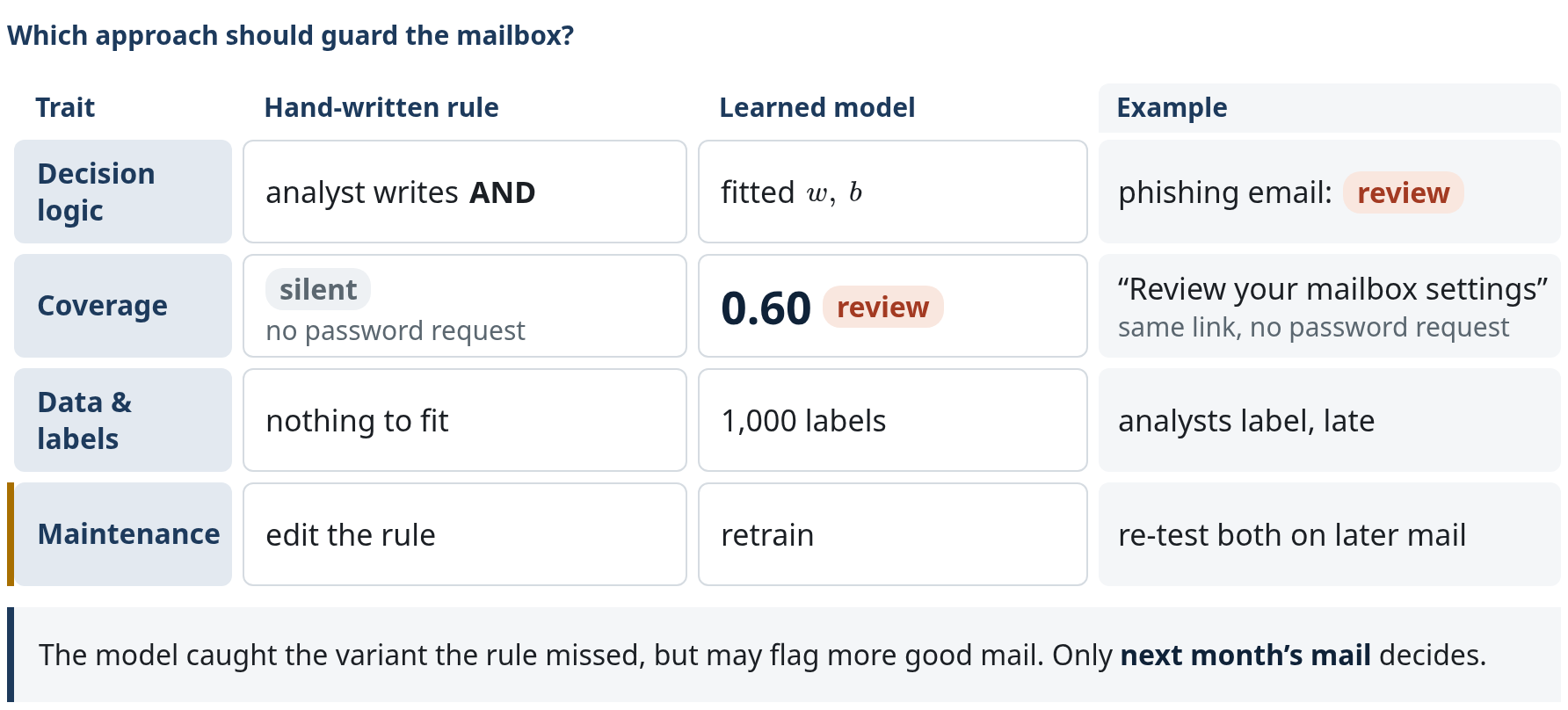
| Trait | Hand-written rule | Learned model | The phishing email |
|---|---|---|---|
| Decision logic | An analyst writes: link mismatch AND credentials? | Fitted from labels: w = (2, 2),\ b = -2 | Both: review; score \sigma(1.0) = 0.73 |
| Coverage | Applies exactly its condition: credentials? no, so silent | Combines partial evidence: z = 2(0.8) + 2(0.4) - 2 = 0.4 | The variant “Review your mailbox settings”: same lookalike link, no password request; rule silent, model 0.60, review |
| Data & labels | No fitting; still needs test emails | Needs data: 1,000 labelled emails | Who labels? Analysts, with delay |
| Maintenance | A new lure: edit the condition | Retrain on new labels: refit w, b | Both: re-evaluate on later mail |
Step by step, as on the slide:
- Decision logic. An analyst writes the rule; the model's weights w = (2, 2) and b = -2 are fitted from labelled emails. On the lure both say review.
- Coverage. The variant “Review your mailbox settings” keeps the same lookalike link but asks for no password, so credential pressure drops to 0.4. The rule’s AND fails and it stays silent; the model scores z = 2(0.8) + 2(0.4) - 2 = 0.4 and \sigma(0.4) = 0.60, still review. The same flexibility lets a model fail on a variant it has not seen.
- Data and labels. The rule needs no fitting but still needs test emails. The model needs data, about 1,000 labelled emails, and analysts supply the labels late and sometimes wrongly. Anomaly methods avoid attack labels for fitting but still need validation.
- Maintenance. A new lure means editing the condition or retraining on new labels. Either way, freeze both, set thresholds on validation data, then compare detection, false alerts and latency on the same future test data. In practice, combine policy rules with learned scoring where that improves the measured result.
Sources: Google, Rules of ML (1, 3, 7, 8, 14, 33) · Sommer & Paxson (2010), on why learned intrusion detectors are harder to deploy than learners in other domains.
Four sources of training signal · slides 17–24
Slide 17 · Four sources of training signal
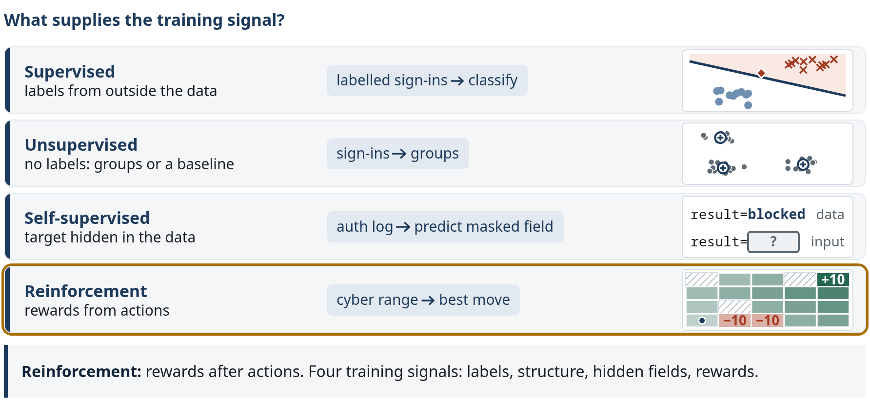
| Setup | Training information | Security example |
|---|---|---|
| Supervised | Inputs with externally supplied labels, here analysts' labels | Is this sign-in an attack? Learn from labelled sign-ins (slide 18) |
| Unsupervised | Inputs without labels; find groups or a baseline | Is this sign-in unusual? (slide 19) |
| Self-supervised | Targets cut from the data itself, such as the next token | Predict the hidden result field of an auth log line (slide 20) |
| Reinforcement | Actions, observations and rewards from interaction | Which host does a red-team agent move to next? (slide 21) |
Step by step, as on the slide:
- Supervised: the labels come from outside the data, here analysts' labels on sign-ins.
- No outside labels. Unsupervised: same kind of sign-ins, no labels; k-means finds three groups, and a group is not an attack label. Then self-supervised: hide the result field of an auth log line and predict it. The record supplies its own target, unlike the externally supplied labels above. Both rows appear on one click; the caption reads: structure, not attack labels; the record supplies its own target.
- Reinforcement: rewards after actions. Value spreads back from the +10 corner of the cyber-range grid. These setups combine; self-supervision is often grouped under unsupervised learning.
The final caption names the four training signals: labels, structure, hidden fields, rewards.
Supervised targets can be categories (classification) or numbers (regression). The large language models in Part 3 are built by self-supervised pre-training followed by supervised and reinforcement fine-tuning. Labels are the scarce resource in security: expensive, delayed and often noisy. That is one reason unsupervised anomaly detection is popular, and one reason it produces many false positives. Sources: Google · Introduction to ML · NIST · Self-supervised learning.
Slide 18 · Supervised learning
Is the 02:14 sign-in an attack? Supervised learning answers from past labelled sign-ins. The axes are failed sign-ins and device novelty, both scaled to 0 to 1. Grey points are unlabelled; the hollow diamond is today's sign-in at (0.46, 0.64). The fit is least squares on 0/1 labels with a 0.5 threshold, the indicator-matrix classifier in Hastie et al. (2009) §4.2:
Step by step, as on the slide (the interactive version below runs the same computation):
- Twenty past sign-ins, not yet labelled, and today's 02:14 sign-in.
- An analyst labels six past sign-ins (filled dots benign, crosses attack). No model yet.
- A line is fitted to the six labels: \mathbf w = (1.185, 0.538), b = -0.494. The 02:14 sign-in scores 0.40, benign side.
- Twelve labels: the line moves, \mathbf w = (0.636, 1.061), b = -0.415, and the same sign-in flips to 0.56: predicted attack. The sign-in did not change; only the labels did.
- All 20 labels: the line settles at \mathbf w = (0.684, 1.050), b = -0.406; the dashed lines are the earlier fits. Substitute the sign-in: 0.684 \cdot 0.46 + 1.050 \cdot 0.64 - 0.406 = 0.58 \geq 0.5, still attack side. The score is not a probability, and it is a prediction, not a confirmed incident.
Good fit: classify records when useful labels exist. Limit: noisy or late labels move the line. Supervised tasks also include regression. Sources: Google · Introduction to ML · Hastie et al. (2009) §4.2.
In the interactive version, Label order shuffles the order in which the labels arrive: the first fits differ, the 20-label fit is the same.
Slide 19 · Unsupervised learning
Same plane as slide 18, but one week of 34 sign-ins and no labels. The only question is whether the 02:14 sign-in is unusual. k-means alternates two moves: assign every point to its nearest centroid, then move every centroid to the mean of its points. It minimises the sum of squared distances
Step by step, as on the slide (the interactive version below runs the same computation, one half-iteration per Step):
- We choose k = 3 and a deliberately poor start, centroids at (0.10, 0.10), (0.20, 0.10) and (0.90, 0.90), then let it run. Two moves repeat: each sign-in joins its nearest centroid, and each centroid moves to the mean of its points. J falls until no point changes group: converged at J = 0.279. Neither move can raise J, so k-means always stops, though another start can stop in a worse local minimum.
- k-means returns groups 1, 2 and 3: 10, 14 and 10 sign-ins. The names, new-device enrolments, routine sign-ins and password-expiry retries, are an analyst's reading of the points. Which group is the attack? Clustering cannot say.
- Anomaly score: distance to the nearest centroid. The largest distance in the training week is 0.139, so the radius is 0.14; the 02:14 sign-in is 0.31 from the new-device group, so it goes to review. Unusual is not malicious; only evidence settles it.
The run inside the first click, iteration by iteration (the J chart on the slide keeps every value): at the start each sign-in joins its nearest centroid and the borders are perpendicular bisectors, J = 7.744. First update: each centroid moves to the mean of its points, then every sign-in is reassigned; ten points change group and J falls to 2.814. Second update: eight points change group, J = 1.272. Third: one point changes, J = 0.292. Fourth: none changes, J = 0.279, converged.
Good fit: group records for exploration and triage, and score distance from a baseline. Limit: a discovered group is not a benign/attack label. Sources: Lloyd (1982) · Chandola et al. (2009), anomaly detection survey · Google · Introduction to ML.
In the interactive version, Start keeps the lecture start or draws random starting sign-ins from a seed. Points that switch group are ringed, and the shaded areas show which centroid is nearest. Try several seeds: k-means can stop in different local minima. The student site's ML playground runs the same code.
Slide 20 · Self-supervised learning
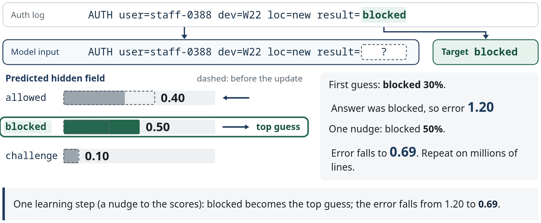
Before anyone labels a sign-in, a model can learn what ordinary auth log lines look like. Take any line from the auth log, here a denied attempt, AUTH user=staff-0388 dev=W22 loc=new result=blocked, and hide its outcome token: the model input ends at result=, and the record itself supplies the target, blocked. No analyst label is needed.
Step by step, as on the slide:
- The model gives every candidate next token a probability, \mathbf p = \operatorname{softmax}(\mathbf z) = (0.60, 0.30, 0.10) for allowed, blocked and challenge. Its top guess, allowed, misses. Real language models normalise over tens of thousands of subword tokens; three keep the arithmetic on one slide.
- Cross-entropy is minus the log of the probability given to the true token: \mathcal L = -\ln 0.30 \approx 1.20. The arrows show the update's direction: more probability on blocked, less on allowed.
- One gradient step on the logits, \mathbf z \leftarrow \mathbf z - 0.7\,(\mathbf p - \mathbf y) with \mathbf y = (0, 1, 0): allowed 0.40, blocked 0.50, challenge 0.10, and the loss falls to -\ln 0.50 \approx 0.69. Repeat at every position in many records.
The “after” values are that one gradient step, rounded to two decimals (exact 0.403, 0.501, 0.095); the gradient of softmax cross-entropy with respect to the logits is \mathbf p - \mathbf y (Goodfellow et al. 2016, §6.2.2.3). Once trained, a high loss on a new line marks a surprising event: that is the link to anomaly detection. Surprise is not an attack label, the outcome token is not a verdict on the user, and next-token prediction is one self-supervised objective among others. Fine-tuning on analyst labels is supervised. Sources: NIST CSRC · self-supervised learning · Goodfellow et al. (2016) §6.2.1.1, §6.2.2.3.
Slide 21 · Reinforcement learning
A red-team agent starts on a workstation in a cyber-range network, a 4 \times 5 grid of hosts: +10 at the backup server, -10 if it touches an EDR-monitored host (the DB and mail servers), -1 per move, discount \gamma = 0.9. Nobody tells it the correct move; it only receives rewards. Value iteration applies one Bellman backup to every host per sweep, starting from V = 0:
Step by step, as on the slide (the interactive version below runs the same computation, one sweep per Step):
- Sweeps 1 to 7: each sweep is one Bellman backup for every host at once, and the +10 spreads one move further back per sweep. After seven sweeps the wave reaches the start at 0.63. The DB and mail servers end the episode at -10 and never pass value on.
- Sweep 8 changes nothing, so the values have converged. Follow the arrows: seven moves through the management server, return G_0 = 0.63.
The sweeps inside the first click: the slide shows each host's value when the wave first reaches it, and that value is already final. Sweep 1: only the host next to the backup server sees the reward, V_1 = \max(+10, -1, -1, -1) = 10; every other host has paid one move. Sweep 2: -1 + 0.9 \cdot 10 = 8. Sweep 3: -1 + 0.9 \cdot 8 = 6.2. Each sweep extends the agent's horizon by one move. Sweeps 4 to 7: 4.58, 3.12, 1.81, then V_7(\text{start}) = -1 + 0.9 \cdot 1.81 = 0.63. Before the wave arrives, synchronous backups give a host -1, -1.9, -2.71, …, because it has only paid moves; the slide skips these transient values.
This agent plans with a known model of the network (value iteration, Sutton & Barto §4.4); learning agents such as Q-learning estimate the same values from experience. \gamma = 0.9 makes later rewards count less (return, §3.3). Reward design is a security decision: an agent optimises the scorer it is given and can learn to game it, as in the Hugging Face breach (slide 68). Sources: Sutton & Barto (2018), §3.3, §4.4 · Microsoft CyberBattleSim, attacker agents in simulated networks.
In the interactive version, Network switches between the current controls and the extra EDR sensor on the management server.
Slide 22 · One sensor changes the route
In plain words: same grid, same 7-move route worth 0.63. A defender adds one EDR sensor on the management server, so the agent takes a nine-move detour worth −1.39. Change the rewards, change the moves it picks.
A defender adds one EDR sensor on the management server. The cheapest route now detours through the lower row: nine moves, value -1.39. Change the rewards, change the policy.
Slide 23 · When does reinforcement learning fit?
| Pros | Cons |
|---|---|
| Optimises action sequences and delayed outcomes. Can encode containment–disruption trade-offs. | Training experience and reward design can be costly. Reward gaming and simulator-to-real transfer failures. |
| Potential good fits: red-team path search or multi-step response in a cyber range (the gridworld); adaptive scan or investigation budgets. | Poor fits / start simpler: one email, phishing or not → classifier baseline; unbounded exploration on critical production systems. |
Step by step, as on the slide:
- Good fit: the gridworld's red-team path search, a multi-step path in a cyber range where each action changes what comes next.
- Start simpler: a single phishing decision on one email is a classifier problem. RL is possible there but is usually an unnecessarily complex starting point; the recommendation is a baseline, not a prohibition.
Answer, as the slide closes: moves change what comes next: RL can fit. One decision per email: start with a classifier.
Decision test: do actions change future outcomes, and can you evaluate that feedback credibly? Offline RL can use logged experience, so RL does not always require exploring a live network; hard action constraints and transfer evaluation still matter. Fit judgements: the lecturer’s, informed by McFadden et al. (2026), USENIX Security (§§4.2, 7.2–7.3, 8.1) and Microsoft CyberBattleSim. Research examples, not production-readiness claims.
Slide 24 · Quick check · which paradigm?
Decide for each task before opening the answer.
Rank the alert queue by learning from analysts' past close / escalate decisions.
Supervised: analysts' decisions are the labels. Labels exist only for alerts analysts saw, so they carry selection bias.
Group 2,000 new lure variants into campaigns nobody has named yet.
Unsupervised: clustering.
Flag a service account that departs from its own history.
Unsupervised / one-class anomaly detection against a (presumed clean) baseline. “Unusual” is learned without attack labels, which is why its alerts need context.
Pre-train on a year of auth logs, then fine-tune with 300 labelled incidents.
Self-supervised pre-training, then supervised fine-tuning.
Choose the red-team agent's next host in the cyber range.
Reinforcement: the agent from the gridworld learns from rewards after its moves, not from labelled correct moves.
From data to a detector · slides 25–28
Slide 25 · Libraries do the maths
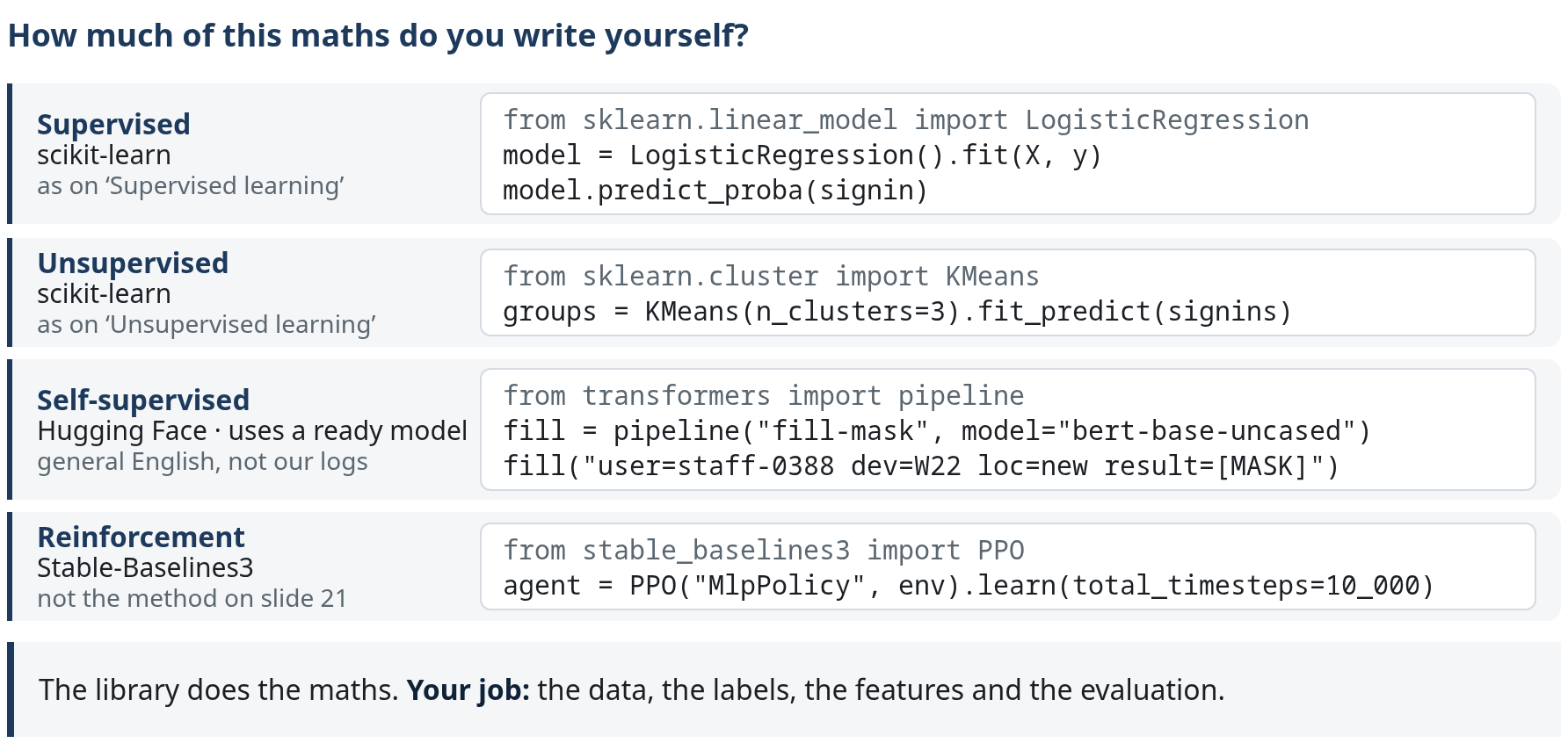
Do you have to write the maths yourself? Almost never. Each paradigm from slides 18–21 is one or two calls to a free, widely used Python library:
- Supervised, as on slide 18, with scikit-learn:
model = LogisticRegression().fit(X, y)fits the weights to labelled emails;model.predict_proba(signin)scores a new one. - Unsupervised, as on slide 19, with scikit-learn:
groups = KMeans(n_clusters=3).fit_predict(signins)runs the whole k-means loop on unlabelled sign-ins. - Self-supervised, as on slide 20, with Hugging Face Transformers:
fill = pipeline("fill-mask", model="bert-base-uncased")loads a model pre-trained by hiding words;fill("user=staff-0388 dev=W22 loc=new result=[MASK]")asks it for the hidden token. - Reinforcement, as on slide 21, with Stable-Baselines3:
agent = PPO("MlpPolicy", env).learn(total_timesteps=10_000)trains an agent in an environment you supply.
Each call needs a line such as from sklearn.linear_model import LogisticRegression first. X, y, email, signins and env stand for prepared feature arrays, labels and a Gymnasium environment with its rewards; preparing them is the real work. We show no output from these calls.
Takeaway: the library does the maths. Your job: the data, the labels, the features and the evaluation. The rest of the lecture is about those four.
Slide 26 · From reported email to alert
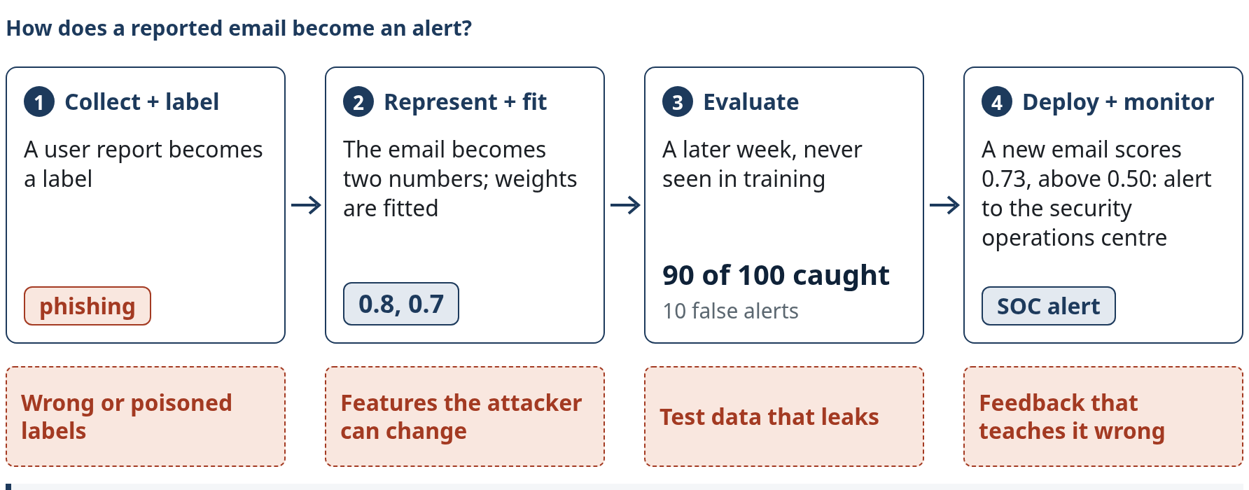
The same phishing email as slide 14, followed through the pipeline. The four stations group the seven stages.
Step by step, as on the slide:
- Collect + label: a user reports the email; an analyst's decision makes it a training label, one of 1,000 labelled emails.
- Represent + fit: the email becomes two numbers, \mathbf x = (0.8, 0.7): link mismatch and credential pressure. Fitting on all labels sets \mathbf w = (2, 2) and b = -2.
- Evaluate: a later week the filter never saw; the token is now a new phishing email with the same two feature values, not the training email. 90 of 100 phishing emails caught, 10 missed, 10 false alerts among 900 legitimate ones. The same counts return on slide 36, at the same 0.50 threshold.
- Deploy + monitor: a new phishing email with the same two feature values: z = \mathbf w^\top \mathbf x + b = 1.0 and \sigma(1.0) = 0.73 \geq 0.50, so it raises a SOC alert. The analyst's decision returns as a label only through the review gate.
- Each stage can fail or be attacked: wrong or poisoned labels; features the attacker can change (slide 27); test data that leaks (Arp et al. P3) or a test with no adaptive attacker (P10); feedback that teaches the model wrong.
The seven stages: collection (source coverage, mutable external data, poisoning) · labelling (analyst evidence versus untrusted feedback) · representation (omitted information, shortcuts, editable features) · training (accepted data, model code, dependencies, backdoors) · evaluation (time splits, untouched tests, operating conditions, attack model) · deployment (manipulated inputs, output leakage, downstream permissions) · monitoring (drift, delayed verdicts, feedback acceptance, retraining and rollback). Completing the seven boxes does not guarantee a secure system. Source: Arp et al. (2022).
Slide 27 · A model sees only what we encode
A model only sees the features it receives: sender authentication, byte patterns, flow timing or sign-in history. Feature engineering encodes domain knowledge; this is where security expertise enters. Missing information creates blind spots.
| Domain | Raw object | Example features |
|---|---|---|
| Phishing | Sender domain age; SPF/DKIM/DMARC results; URL length and lookalike domains; urgency words; HTML forms | |
| Malware (PE files) | Executable | Byte histograms; section entropy; imported API functions; header fields; strings |
| Network | Flow records | Bytes and packets per direction; duration; ports; inter-arrival times; periodicity |
| Identity | Sign-in logs | Time of day; device and location novelty; failed attempts; impossible travel |
Engineered PE-file features: Anderson & Roth (2018), EMBER [preprint].
Predict: what can an attacker do to a text-only phishing detector? Answer before opening.
Answer, as revealed on the slide
- The same lure arrives as an image with a QR code. The text extractor finds no text, so both features read 0: 2(0) + 2(0) - 2 = -2 and \sigma(-2) = 0.12 \lt 0.50: delivered. The model did not change; the score fell from 0.73 to 0.12.
- An OCR and QR decoder before the features recovers
mail.exampIe.com/resetand restores 0.73, review. It costs compute and adds a component the attacker can target. - What is not represented cannot be detected; what is represented can be manipulated. The final state keeps the failure beside the repair: a dashed tag “text only: 0.12 → delivered” stays beside “review”, and the caption reads Same lure, new representation: 0.12 as text only, 0.73 once decoded. A richer model, the gateway's v2, adds sender-domain age, urgency, spelling and password-form features: it scores this lure 0.97. The later 0.97 is a different model, not a contradiction.
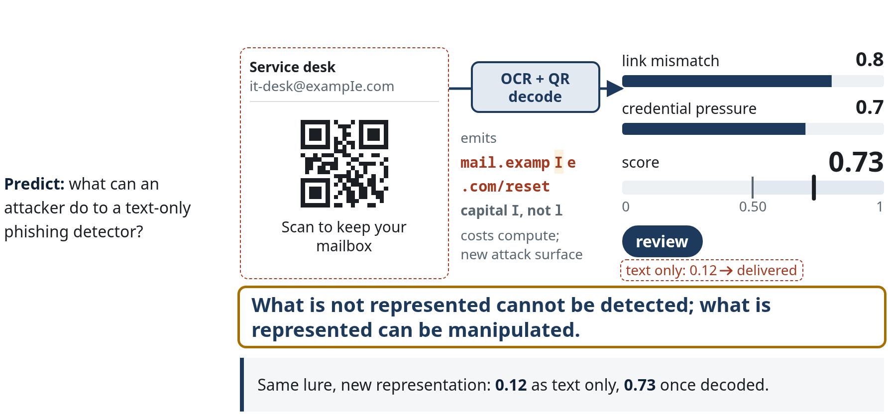
Treating a feature that cannot be computed as 0 is a modelling choice; a pipeline could mark it missing instead. Representation choices define the evasion space.
Further practice with a different representation: Lab 13 learns from 64 pixel brightness values instead of supplied clues.
The input is 64 pixel brightness values. Can recognising the mark establish that the page is safe?
No. The model learns the supplied review labels from an 8-by-8 image. The image does not include who owns the page or approved the workflow.
Slide 28 · Three model families, one file
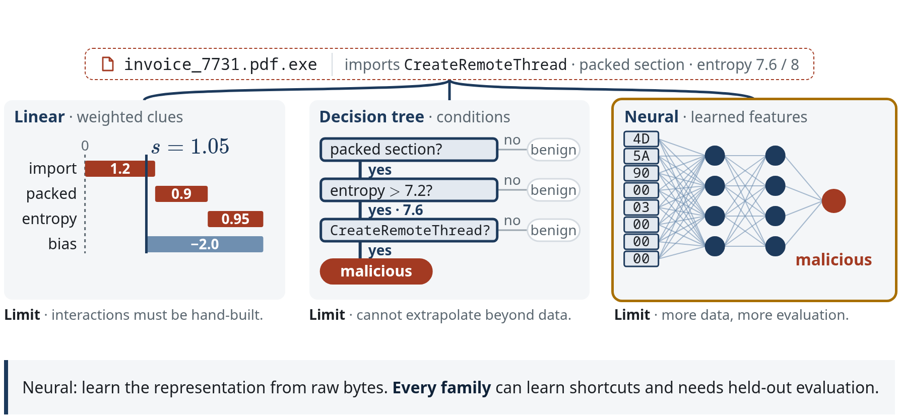
One attachment, invoice_7731.pdf.exe; one file, three model families.
Step by step, as on the slide:
- Linear: each feature times its weight adds to the score. The CreateRemoteThread import adds 1.2, the packed section 0.9, section entropy 7.6 of 8 (0.95) adds 0.95; the bias of -2.0 pulls the total back to s = \mathbf w^\top \mathbf x + b = 1.2 + 0.9 + 0.95 - 2.0 = 1.05 > 0: malicious. A contribution is relative to the feature representation, and a score is not automatically a calibrated probability.
- Tree: follow conditions to a leaf. Packed section? Yes. Entropy above 7.2? Yes, 7.6. Imports CreateRemoteThread? Yes: malicious. A tree ensemble votes or averages over many such trees. Each leaf is a constant, so the ensemble cannot extrapolate beyond the feature ranges seen in training (Hastie et al. 2009, §9.2, §10). Trees do not guarantee faithful or simple explanations.
- Neural: no hand-made features. The first header bytes,
4D 5A 90 00 03 00 00 00, go in raw, and the layers learn their own representation (Raff et al. 2018). Neural models are not automatically superior: on tabular features tree ensembles often match or beat them (Grinsztajn et al. 2022), and they cost more data and evaluation.
| Linear · weighted clues | Decision tree · conditions | Neural · learned features | |
|---|---|---|---|
| Limit | Interactions must be hand-built. | Cannot extrapolate beyond the data. | More data, more evaluation. |
Every family can learn a shortcut, a spurious correlation in the training data, so each needs held-out evaluation (Arp et al. 2022). Sources: Grinsztajn et al. (2022) · Raff et al. (2018) · Hastie et al. (2009) §9.2, §10.
How a model learns · slides 29–33
Slide 29 · How a model learns
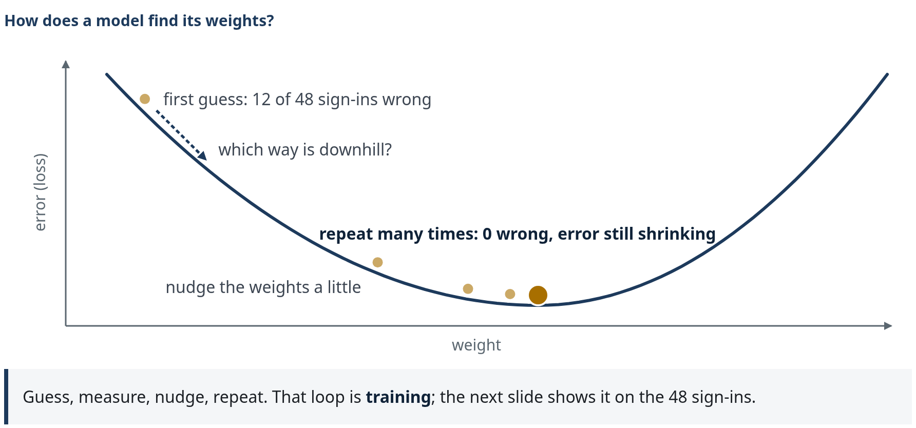
How does a model find its weights? Picture the error as a valley over one weight: each possible weight gives some number of mistakes on the training data, and training looks for the lowest point.
Step by step, as on the slide:
- First guess. Start from some weights. On the sign-in data of slide 30 the first guess gets 12 of 48 sign-ins wrong.
- Which way is downhill? Measure how the error changes when the weight moves a little. That slope is the gradient.
- Nudge. Take a small step downhill. The faint dot marks where the ball was.
- Repeat. Measure and nudge again; the steps shrink as the ground flattens. Training stops when the error stops improving: 0 wrong.
Guess, measure, nudge, repeat: that loop is training. A real model has many weights, so its valley has many dimensions, and slide 30 measures a smooth loss rather than counting mistakes; the loop is the same. Source: Goodfellow, Bengio & Courville (2016) §4.3.
Slide 30 · Learning is optimisation
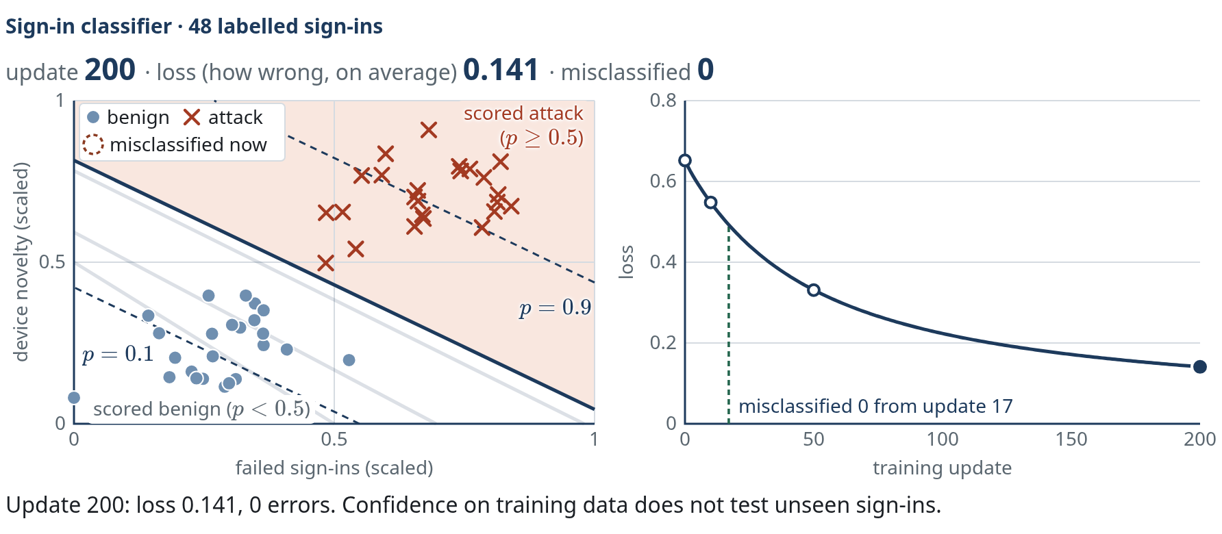
The same loop as slide 29, now on a real classifier. Two features, failed sign-ins and device novelty, so we can draw it; real models use hundreds or millions of dimensions, but the mechanism is the same. The boundary is the line where the score p = 0.5. Zero training errors is not the end: the loss also measures confidence.
Step by step, as on the slide:
- Update 0: the starting weights misclassify 12 of 48 training points (dashed rings). Loss 0.652.
- Update 10: each small step on the weights lowers the loss. The boundary shifts towards the attacks and tilts slightly; 6 errors remain. Loss 0.548.
- Update 50: no training errors since update 17, yet the loss (0.331) is still falling. If nothing is misclassified, what is still being optimised?
- Update 200: loss 0.141, still 0 errors. The lower loss means more confident scores on the training points, not evidence about unseen data: same decisions, steeper scores. The dashed p = 0.1 and p = 0.9 contours show it.
Background: confident on training data is still fragile near the boundary. The attack closest to the final boundary scores p = 0.58. Lower its device novelty by 0.06 and it scores p = 0.49: scored benign. Points near the boundary are uncertain and cheap to push across. This is a hypothetical edit; the open question is which features an attacker actually controls (Biggio et al. 2013).
Behind the slide, not shown on it: logistic regression scores p = \sigma(\mathbf w^\top \mathbf x + b), the cross-entropy loss is
and full-batch gradient descent updates \mathbf w \leftarrow \mathbf w - \eta \nabla \mathcal L with learning rate \eta = 0.8: each update works out which way to change \mathbf w and b to lower the loss, takes a small step and repeats. At update 200, \mathbf w = (4.311, 5.597) and b = -4.561; 25 of 48 points lie beyond the p = 0.1 and p = 0.9 contours, against 0 at update 50, and \lVert \mathbf w \rVert went from 3.2 to 7.1. On separable data the loss only reaches 0 as \lVert \mathbf w \rVert \to \infty, which is why we stop early or regularise (Goodfellow et al. 2016 §7.3, §7.8).
Sources: Goodfellow, Bengio & Courville (2016) §4.3, §5.7.1, §7.3, §7.8 · Biggio et al. (2013).
Slide 31 · Training, validation and test data
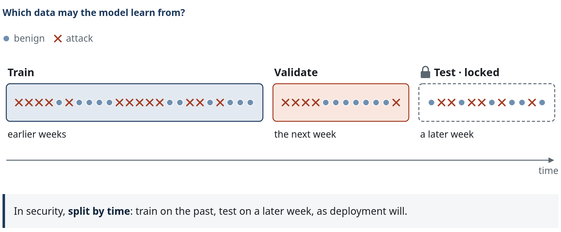
Which data may the model learn from? On slides 29 and 30 the model trained on every labelled sign-in. A real project splits its labelled examples into three parts with different jobs.
Step by step, as on the slide:
- Training data, the largest part: the model fits its weights here.
- Validation data, a second slice: compare settings, such as model size or the review threshold, and keep the best.
- Test data, the last slice, locked: used once, at the end, to estimate performance on unseen data. The test set must not influence any choice. If you pick features, a model size or a threshold by looking at test error, the test set has become a second validation set, and its error underestimates the error on new data.
- Split by time. Clicks 1 to 3 split at random. In security, train on earlier weeks, validate on the next week and test on a later week, as deployment will. A random split lets the model train on samples from after the ones it is tested on, which inflates results (temporal bias; Part 3 returns to this).
Hastie et al. give 50% training and 25% each for validation and test as a typical split; the right sizes depend on the noise in the data and the number of examples. Slide 32 uses validation error to catch overfitting. The week labels are an analogy, like the months on slide 32.
Sources: Hastie, Tibshirani & Friedman (2009) §7.2 · Pendlebury et al. (2019).
Slide 32 · Validation catches overfitting
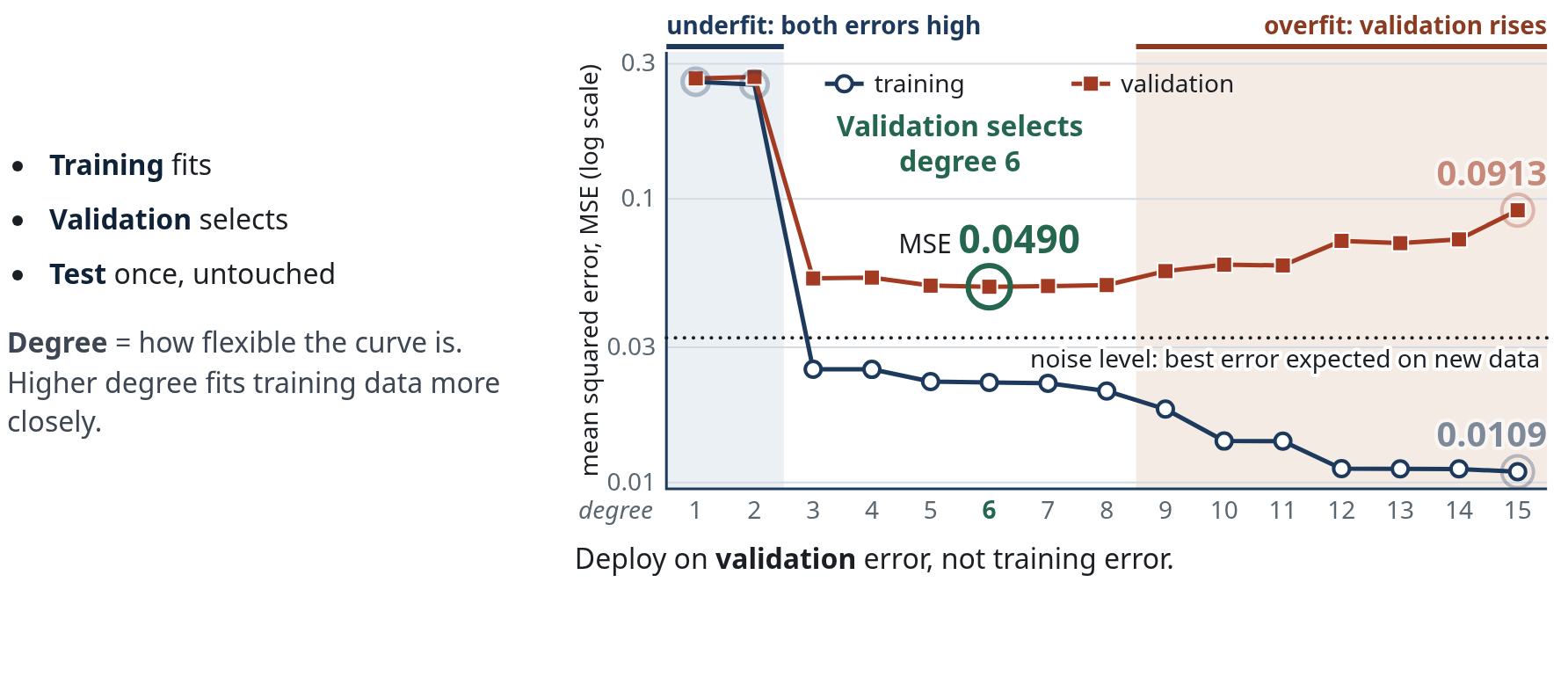
- Use training data to fit parameters, validation data to select the model, and an untouched test set for the final evaluation.
- Extra complexity can fit training noise while validation error rises: overfitting. A model too simple for the pattern underfits.
- Security example: train on mail before July, select on July, then test once on a later, untouched window: August.
Mean squared error (MSE) averages the squared gaps between predictions and supplied values. Step by step, as on the slide:
- Training MSE falls with every added degree: 0.259 at degree 1, 0.0109 at degree 15. Which degree would you deploy?
- Validation MSE on 500 independent points: about 0.26 at degrees 1–2 (both errors high: underfit), 0.049 to 0.053 at degrees 3–8, rising from degree 9 to 0.0913 at degree 15 (overfit).
- Noise variance \sigma^2 = 0.18^2 = 0.0324 (dotted line). Degree 15 reaches training MSE 0.0109, a third of that, while validation rises: the extra fit is noise. This is not a rule that any training error below \sigma^2 proves overfitting: least squares with p parameters on n points has expected training error \mathbb E[\text{train MSE}] = \sigma^2 (1 - p/n) even when the model is right, 0.021 for degree 6 (p = 7) and 0.0065 for degree 15 (p = 16). Only the rising validation curve shows overfitting (Hastie et al. 2009 §7.4).
- Validation selects degree 6 (MSE 0.0490), the lowest recorded validation value in this run, not a test result. Degrees 5–8 lie within one standard error (0.0031) of the minimum, so the one-standard-error rule picks the simplest, degree 5 (Hastie et al. 2009 §7.10).
- Security version: train on mail before July, validate on July, keep August locked for the final test. No test result is shown. “Unseen” in deployment means future data from adaptive adversaries; a random split can answer an easier question (Part 3, Pendlebury et al. 2019). The months are an analogy, not the source of this polynomial data.
Sources: Hastie, Tibshirani & Friedman (2009) §7.2, §7.4, §7.10 · Goodfellow et al. (2016) §5.2–5.3 · Pendlebury et al. (2019).
Slide 33 · Demo · fitting a score versus choosing a review threshold
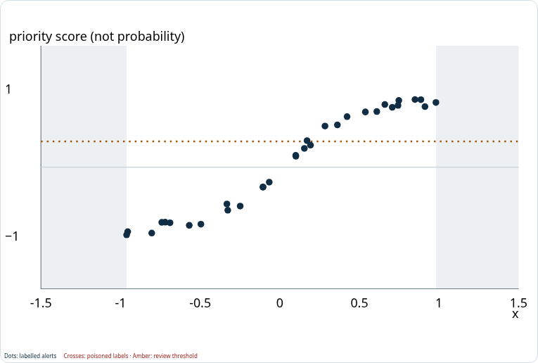
The lecturer drives Lab 01 on the projector for about eight minutes:
- Fit: a straight line, then a small neural network.
- Check: validation mean squared error (MSE).
- Decide: freeze the weights; change the review threshold.
Predict: which changes the fitted curve: training or moving the threshold? Lab 01 predicts a priority score (regression), so the “boundary” there is a threshold on a score curve, not a line between two classes as on slides 18 and 30. Repeat the demonstration yourself:
Which changes the fitted curve: training or moving the threshold?
Training changes the weights and therefore the fitted curve. The threshold only changes which fixed scores enter review.
Core route in the lab: straight line with w = 0 and b = 0, then b = 0.50 and w = 1; press One update once. Then choose Clean triage labels, Neural network · 12 hidden units, Reset, Train 1,000 steps and record the validation MSE. Keep the model fixed and compare thresholds 0.15 and 0.70: false alerts (false positives, FP), missed priority alerts (false negatives, FN) and queue size. Those two error types become the confusion matrix in Part 2.
Go deeper with Lab 01 · worked numbers
Feature and label. Usual window 4 failed logins, now 6; with one input unit = 4 extra attempts, the input is (6 - 4) \div 4 = 0.5. The supplied teaching answer (label) is priority 0.6. Both scales are teaching choices, and the priority is not an attack probability.
Weight and bias. Score = w x + b. With x = 0.5: 1 \cdot 0.5 + 0 = 0.5; 1 \cdot 0.5 + 0.2 = 0.7 (the bias shifts every output); 2 \cdot 0.5 + 0 = 1.0 (the weight changes how strongly the output responds). Weights and biases are the model's parameters.
One update. With bias 0, weight 0.4 gives 0.2 (0.4 below the label 0.6); weight 0.8 gives 0.4 (gap 0.2). Squared error 0.4 \cdot 0.4 = 0.16; averaged with another squared error of 0.04 gives MSE 0.10. One weight affects many examples, so training reduces the average error; validation then checks separate examples without updating on them. The lab uses the Adam optimiser, which does not guarantee a global optimum.
Capacity. The 12-unit network has 12 input weights, 12 hidden biases, 12 output weights and 1 output bias: 37 parameters. It can follow curved patterns a line cannot, and it can also fit noise.
Threshold. Four alerts (0.20 normal, 0.40 priority, 0.60 normal, 0.80 priority): at threshold 0.50, 0.60 is a false alarm, 0.80 a correct review and 0.40 a miss. Raising the threshold to 0.70 drops the false alarm but still misses 0.40; the scores do not change.
Beyond the training range. A recorded reference run of the clean 12-unit model returns about 0.909 at x = 1.20, outside the training range -1 to 1. This is inference with fixed weights; a returned number is not evidence of accuracy there. Keep the held-out test sealed until model, updates and threshold are recorded: training questions, rehearsal questions and a sealed exam.
Concept reference: Goodfellow, Bengio & Courville (2016), ch. 5.
Self-check · Part 1
Part 1 answer · How does a model learn from data? Labels, structure, hidden fields or rewards, on our features.
Typical label sources and their weaknesses
Analyst verdicts (delayed, inconsistent), user reports (noisy, manipulable), vendor verdicts (aggregated, lagging). The second question stays open.
You train for more steps, then move the threshold from 0.50 to 0.70. Which action changes the fitted curve?
Training: it changes the weights. Moving the threshold changes only which fixed scores reach review (slides 14 and 33).
The 02:14 sign-in scores 0.40 after six labels and 0.56 after twelve. What changed?
Only the labels. The sign-in is the same point; the least-squares fit moved because more labels arrived (slide 18).
k-means puts the 02:14 sign-in 0.31 from the nearest centroid, beyond the 0.14 radius. Is it an attack?
Not established. It is unusual for this week of sign-ins, so it goes to review. Clustering cannot say which group is the attack; only evidence settles it (slide 19).
Which paradigm learns from rewards rather than labels?
Reinforcement learning. A reward evaluates an outcome after an action; it is not a correct-action label. One extra sensor changed the agent's best route and its value from 0.63 to -1.39 (slide 21).
Why can validation error rise while training error keeps falling?
The extra complexity fits noise in the training sample. On slide 32, degree 15 reaches training MSE 0.0109 while validation MSE rises to 0.0913: overfitting.
A text-only filter scores the lure 0.73. The attacker moves the text into a QR image. What is the score, and why?
About 0.12: both text features become 0, so 2(0) + 2(0) - 2 = -2 and \sigma(-2) \approx 0.12. The representation, not the model, was bypassed (slide 27).
Practise Part 1
Notebook: Lesson 1 · Teach a login-alert model. Worked examples: Lesson 1.